I just posted a function that fits a variant of the diversity-dependent phenotypic evolution model that we used in Mahler et al. (2010). The function is called fitDiversityModel() and it is available on my R-phylogenetics page (direct link to code is here).
Both the model and the function are very simple. Basically, we scale the rate of evolution along the branches descending from each node by the estimated lineage density at that node. The user can supply a vector of lineage densities, or the function can estimate lineage density by merely counting the number of branches in the tree at the time of the node in question. The latter option, obviously, does not take into account extinction or incomplete taxon sampling. The assumption implicit in scaling branches in this way is that variation in the rate of phenotypic evolution among branches is entirely determined by lineage densities at the origin of each branch!
The way I implemented this in practice was straightforward. I merely rescaled the branches of the tree based on estimated or supplied lineage density, and then maximized the likelihood of the scaling parameter and starting rate given the data. I also allow the user to visualize this branch length rescaling with the option showTree=TRUE.
In the process of adding error handling to this function I also made a curious realization about extracting vectors from data frames and matrices that I thought might be of interest to some readers.
Consider the following matrix:
> X
V1 V2
A 0.949 1.062
B 1.248 1.375
C -0.835 1.047
If we want to extract "V1" we can just type:
> v1<-X[,1]
> v1
A B C
0.949 1.248 -0.8355
Here, v1 inherits the row names of X. By contrast, if X is a data frame:
> X<-as.data.frame(X)
> X
V1 V2
A -0.264 0.100
B 0.026 -1.961
C -1.408 -0.205
> v1<-X[,1]
> v1
[1] -0.264 0.026 -1.408
In this case, although the operation on X is identical, v1 does not inherit the row names of X as its names! Tricky.
Tuesday, April 26, 2011
General comments page
I just added a dedicated "Comments" page (see link above). Hopefully this will serve as a place for general comments about the blog, as well as questions or suggestions pertaining to any of the functions posted to my R-phylogenetics page. Please comment!
Monday, April 25, 2011
Small updates to evol.rate.mcmc()
A couple of additional small updates to the function evol.rate.mcmc(). Direct link to code (v0.4) is here.
1) Now the user can specify the starting values for σ(1)2, σ(2)2, and a. This comes in response to a reviewer comment and I think it is a really good idea because one should be sure that the MCMC will converge to the correct distribution (eventually) regardless of where it is started. Now that will be easy to demonstrate. Starting values for the MCMC can be set using the control parameter list, e.g.:
> result<-evol.rate.mcmc(...,control=list(sig1=100,sig2=100,a=0))
If no starting values are supplied, the default setting should give the user starting values on the correct order of magnitude (which still seems like a good idea).
2) In my initial version of the raw MCMC result pre-processing function, posterior.evolrate(), I had the function plot the stretched or contracted tree for every generation of the chain. This was used to create my animation is a prior post (here). Obviously, this will be slow and annoying feature for large trees and long chains! It can now be turned on or off using:
>mcmc<-posterior.evolrate(...,showTree=TRUE)
(the default is off, i.e. showTree=FALSE ).
That's it!
Sunday, April 24, 2011
Updates to evol.rate.mcmc() & new analysis of the posterior sample
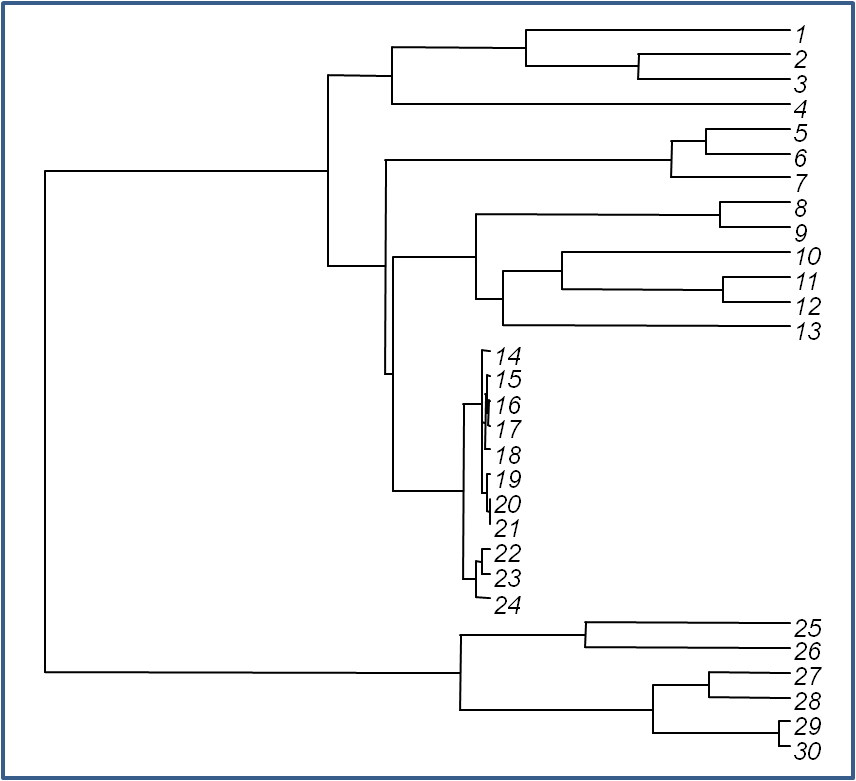
I just posted a new version of evol.rate.mcmc(), our MCMC method for identifying the location of a shift in the evolutionary rate through time. I described this method in a previous post here and in an upcoming publication with several coauthors (1,2,3). In the original version of this function, I had some peculiar bookkeeping. For instance, I defined the derived rate as σ(1)2 if it was left of the root; and as σ(2)2 if right of the root. This was to try and avoid ending up with a posterior sample consisting of a mixture of the two rates. The biggest addition in the present version is a a post-hoc processing of the posterior sample which helps negate this problem entirely (and thus removes the necessity of "anchoring" σ(1)2 or σ(2)2 to the left or the right side of the tree, respectively). The method basically works as follows. First, I use my function min.split() to find the "median" shift point in the tree. Here, I define this as the posterior sample with the minimum summed patristic distance to all the other sampled points on the tree. Next, I use the function posterior.evolrate() which takes this average shift point and the raw posterior sample, and then returns for each posterior sample the mean rate upstream and downstream of the average shift. I did this as follows: 1) For sample i, I split the tree at shift point i; 2) I then scaled each side of the split tree by their respective rates; 3) Next, I reattached the two sides of the tree; 4) Finally, I split the tree at the mean shift point and computed the evolutionary rates upstream and downstream of this split. The figure below shows the tree from my simulated example dataset here, where the branches of the tree have been scaled by the estimated rates. Code for these analyses is on my R-phylogenetics page (direct link here). To run on the dataset from my previous post, please try the following code:
> require(ape)
> tree<-read.tree(text="((((30:0.014,29:0.014):0.171,(28:0.109,27:0.109):0.076):0.258,(26:0.275,25:0.275):0.168):0.557,(((((24:0.238,(23:0.139,22:0.139):0.099):0.199,((((21:0.009,20:0.009):0.045,19:0.054):0.08,(18:0.083,((17:0.043,16:0.043):0.008,15:0.051):0.032):0.051):0.007,14:0.141):0.297):0.095,((13:0.386,((12:0.089,11:0.089):0.216,10:0.306):0.08):0.035,(9:0.095,8:0.095):0.326):0.111):0.009,(7:0.159,(6:0.112,5:0.112):0.047):0.383):0.078,(4:0.535,((3:0.203,2:0.203):0.151,1:0.354):0.181):0.085):0.38);")
> x<-c(6.017,4.73,7.254,11.821,10.391,12.794,15.405,7.941,5.78, 12.71,11.199,10.748,11.927,9.615,9.248,8.973,9.055,9.095,9.892, 9.818,9.838,8.355,8.672,8.972,9.177,5.782,4.762,6.763,1.575,1)
> names(x)<-as.character(1:30)
> source("evol.rate.mcmc.R")
> result<-evol.rate.mcmc(tree,x,ngen=100000,control=list(sdlnr=2))
> minsplit<-min.split(tree,result$mcmc[201:1001,c("node","bp")])
> mcmc<-posterior.evolrate(tree,minsplit,result$mcmc[201:1001,], result$tips[201:1001])
To plot the tree with branch lengths rescaled to the estimated rate, try:
> ave.rates(tree,minsplit,extract.clade(tree, node=minsplit$node)$tip.label,colMeans(mcmc)["sig1"], colMeans(mcmc)["sig2"],minsplit)
which should return a plot much like the one below:
Friday, April 22, 2011
MCMC method: more on analyzing the posterior sample
I've been working a little more on analyzing the posterior sample from our Bayesian MCMC method for identifying the location of a single shift in the evolutionary rate for a continuously valued character. I originally described this method (which has also been submitted for publication with several coauthors) on the blog here. I'm not done with this, but I created an animation of 801 samples from the posterior distribution created by a 100,000 generation MCMC run on the simulated dataset and tree given here. In the animation, the branches of the tree are stretched or shortened depending on their relative rates for that sample. You can see that most of the posterior density for the rate shift is on the generating edge, but that some samples occasionally stray to different parts of the phylogenetic tree. I will be updating the code for all of these analyses very soon.
I have to admit that this animation is not nearly as neat my animation of all bi- and multifurcating trees (although at least it is shorter). I recommend watching it with Robert Randolph "Jesus is Just Alright" playing in the background (as I did). It will surely seem cooler that way.
I have to admit that this animation is not nearly as neat my animation of all bi- and multifurcating trees (although at least it is shorter). I recommend watching it with Robert Randolph "Jesus is Just Alright" playing in the background (as I did). It will surely seem cooler that way.
Brian O'Meara phyloseminar
 I just realized today that I somehow missed Brian O'Meara's phyloseminar - and not just barely, but by 3 weeks! On March 30th, Brian spoke about applying the methods of ABC (Approximate Bayesian Computation) to phylogenetic comparative biology. This is a really neat new area in our field and Brian is sure to put out some interesting publication on this over the next few years.
Luckily, it is still possibly to watch the recording of Brian's seminar which is available (presumably in perpetuity) here. Today during lunch I had time to watch only the first 1/2 of this recording, but I plan to watch the rest of it soon.
Wednesday, April 20, 2011
Phylogenetic RMA regression
I just posted a function that I wrote a while ago (and updated today) for phylogenetic reduced major axis (RMA) regression. The function is available on my R-phylogenetics page (direct link here).
The calculation of the RMA regression slope is straightforward. It is described in Ives et al. (2007). Basically, to get the slope we just compute the phylogenetic variance of y & x and then take the square root of their ratio.
I.e., for phylogeny tree, and vectors x & y in order tree$tip.label:
> C<-vcv.phylo(tree)
> ax<-sum(solve(C,x))/sum(solve(C)) # phylogenetic mean for x
> ay<-sum(solve(C,y))/sum(solve(C)) # same for y
> beta1<-sqrt(t(y-ay)%*%solve(C,y-ay)/(t(x-ax)%*%solve(C,x-ax)))
To get the intercept, we just plot through the phylogenetic means:
> beta0<-ay-beta1*ax
My function also (optionally) optimizes Pagel's lambda & computes the residuals in the y dimension. When I get a chance I will add hypothesis testing of beta0 & beta1 following Ives et al. (2007).
Tuesday, April 19, 2011
Problem with bind.tree()
Today I ran into a slight problem with the {ape} function bind.tree(). I posted this issue to the R-sig-phylo email listserve. Emmanuel Paradis, the author of {ape}, is normally excellent at responding to queries like this - but in the meantime I thought I would also describe the issue in this forum.
I said in my listserve post: "For some reason, when I bind a tree with a root.edge to a tip, the length of the edge leading to that tip is attached not only to the root.edge of the bound subtree, but also to another tip of the tree." Actually, this is imprecise. In fact, the edge length from the edge leading to the target tip is for some reason moved to another tip in the tree.
The easiest way to illustrate this problem is with an example.
First, take the following tree:
text="(1:3.785,(((((8:0.13,9:0.13):0.205,6:0.335):0.154,(10:0.278,7:0.278):0.211):0.1,(4:0.386,5:0.386):0.203):2.655,(2:1.08,3:1.08):2.164):0.54);"
tree<-read.tree(text=text)
plot(tree)
edgelabels(round(tree$edge.length,2),adj=c(0.5,-0.2),frame="none")
Which produces the plot below in which I have labeled edges with their (rounded) lengths:

Now to reproduce our issue, let's cut out the clade with tips "2" and "3", and then regraft it in the same place:
node<-19 # this is the node we will extract
position<-1.0 # this is the length of the root.edge
# extract clade and attach root edge
tr1<-extract.clade(tree,node=node); tr1$root.edge<-1.0
x11(); plot(tr1,root.edge=T) # plot the extracted clade
edgelabels(round(tr1$edge.length,2),adj=c(0.5,-0.2),frame="none")

The length of the root edge is not shown, but remember we have set it to be 1.0.
# now remove tips in tr1 from tree
tr2<-drop.tip(tree,tr1$tip.label,trim.internal=FALSE)
# subtract root.edge of tr1 from tip ending in "NA"
temp<-match(which(tr2$tip.label=="NA"),tr2$edge[,2])
tr2$edge.length[temp]<-tr2$edge.length[temp]-position
x11(); plot(tr2,root.edge=T) # plot the pruned tree
edgelabels(round(tr2$edge.length,2),adj=c(0.5,-0.2),frame="none")

Here is the tree with clade (2,3) extracted.
# now bind tr1 to tr2, where it was removed
tr.bound<-bind.tree(tr2,tr1,where=which(tr2$tip.label=="NA"))
# now plot, to visualize the result
x11(); plot(tr.bound)
edgelabels(round(tr.bound$edge.length,2),adj=c(0.5,-0.2),frame="none")

So, for some reason the edge leading to "NA" before we use bind.tree(), is actually moving to taxon "5" when we reattach the subtree with species "2" and "3". Weird.
Please let me know if you can repeat this error; or, even better, if you figure out that I have made some kind of mistake in my example, above. Thanks!
In a future post (hopefully soon, if I can get this figured out) I will describe what I have been using extract.clade() and bind.tree() for today as it may be of interest to some readers.
Friday, April 15, 2011
Updates to phylosig()
I made a few updates to my function phylosig(), which computes phylogenetic signal using two different methods (method="K" and method="lambda"); and can also conduct hypothesis tests of the null hypothesis that phylogenetic signal is absent. I have posted this function on my R-phylogenetics page (direct link to code here).
Most of the updates are designed to allow the function to accept data vectors with missing data (either as missing elements in the vector, or as NA); as well as data vectors that contain data for species not represented in the tree. In the former case (where we have tips in the tree that are not in the data vector), I use drop.tip() from the {ape} package to remove these tips; and in the latter case (where we have data for tips not present in the tree), we simply excise these data elements from our vector. In both cases, an informative message is triggered. Thanks to Christofer's comments on my previous post for inspiring these improvements.
The other update allows the function to return lambda>1.0. There was some discussion about the theoretical maximum for lambda on the R-sig-phylo email listserve (e.g., here and subsequent messages). I now first compute the maximum possible value for lambda (this is the maximum value for lambda for which the likelihood expression is still defined), as follows:
maxLambda<-max(C)/max(C[upper.tri(C)])
And then I optimize lambda for the interval (0,maxLambda):
res<-optimize(f=likelihood,interval=c(0,maxLambda),y=x,C=C,maximum=TRUE)
This seems to work fine. [Note that I believe that the likelihood expression will be defined from -maxLambda to maxLambda, so if we wanted to allow the possibility of lambda less than 0 we could easily add that here.]
Wednesday, April 13, 2011
Small change to optim.phylo.ls()
I just made a small change to the least-squares phylogeny inference function optim.phylo.ls() (v0.3) in which I test if the input matrix is an object of class "dist" and if so, convert it to a matrix, i.e.:
if(class(D)=="dist") D<-as.matrix(D)
This is useful because the {ape} function dist.dna() actually creates a lower-triangular distance matrix object, that will not work with my function [although the conversion is easy, as evident above].
if(class(D)=="dist") D<-as.matrix(D)
This is useful because the {ape} function dist.dna() actually creates a lower-triangular distance matrix object, that will not work with my function [although the conversion is easy, as evident above].
Tuesday, April 12, 2011
Fixes and improvements to phyl.pca()
I have posted a couple of fixes and improvements to phyl.pca().
First, the original function had a small bookkeeping bug - that has been fixed.
However, more significantly, I made a number of improvements to the function that cut the run-time on a sample dataset by better than 1/2.
First, I added some front-end error checking that I have been trying to incorporate into some of my functions. Here, I check to see if the data (in Y) have rownames, and if the rownames match the tree tip labels. In addition, however, I also allow an incomplete match, so long as all names in Y are found in the tree. To accomplish this, I just retain or prune rows and columns from C<-vcv.phylo(tree) based on their presence or absence in Y. That is:
C<-vcv.phylo(tree)[rownames(Y),rownames(Y)]
Next, I tried to improve the computational performance of the function. I did this in a few different ways. I minimized the number of calls to the {ape} function vcv.phylo() - which can be quite slow. I did this by first computing C<-vcv.phylo(tree), and then passing C, not the phylogeny, to phylo.vcv() [my function to compute the evolutionary variance-covariance matrix among traits] and likelihood() [my function to compute the likelihood for method="lambda"].
Finally, and this had the biggest impact of all, I halved the number of times I had to compute the n*m × n*m Kronecker product of C & R<-phylo.vcv(...)$R; and, wherever it made sense, I switched out solve(A)%*%B in favor of solve(A,B) [as suggested by Vladimir Minin]. The number of times I could do this was fairly small, as I had previously discovered that although solve(C,X) is faster than solve(C)%*%X, as suggested by Vladimir, if we have to compute invC<-solve(C) anyway, then invC%*%X becomes faster than solve(C,X). That said, I was able to use his suggestion with the largest matrix in the analysis (that is, the aforementioned Kronecker product). This certainly helped a lot because for each call of solve(A,b) (instead of solve(A)%*%b) in our likelihood function, we save nearly 3/4 of a second.
The updated function (v0.2) is on my R-phylogenetics page (direct link to code here).
Monday, April 11, 2011
New function: phyl.pca()
I just posted a new function for phylogenetic principal components analysis (as described in my 2009 paper, here). In my article, I gave R code to do this as an appendix; however, this new function expands on that originally very simple function by eliminating some preliminaries (e.g., the operation vcv.phylo(...), for instance), as well as by adding the estimation of joint lambda (by way of method="lambda") for the variables in our input matrix.
The function is available on my R-phylogenetics page (direct link to code here).
To use, just load the function from source:
> source("phyl.pca.R")
then type:
> result<-phyl.pca(tree,X,method="lambda",mode="corr")
(or some variant thereof, depending on the settings desired.)
Unfortunately, likelihood estimation using method="lambda" is pretty slow. I have tried to speed it up a little by minimizing the number of calls to solve(...) and use of the matrix operator %*%. Note that optimization time here scaled with the number of taxa × the number of traits (rather than just with n, as in phyl.resid()).
I did this a couple of different ways. First, I simply avoided multiple calls to solve(C) whenever possible by first setting invC<-solve(C). Unfortunately, optimization of lambda using likelihood requires constant readjustment of C, so this probably had pretty limited impact. Second, I substituted the calculation sum(invC) for the matrix operation 1'C-11 and colSums(invC%*%X) for 1'C-1X.
At some point I will try to update this using functions from the package {Matrix} which I'm told are considerably faster than the matrix operators in R {base}. When I get around to this I will report the result!
For more details on this analysis - I refer the reader to my paper.
Wednesday, April 6, 2011
All furcating trees
Brian O'Meara posted a while ago to R-sig-phylo that he was looking for code to find all bi- and multifurcating rooted trees for a set of taxa. I realized that a function to generate all unrooted trees would be straightforward to program using my add.everywhere() function described previously. [Adding rootedness should then merely involve going through each tree and placing the root along each edge.]
I ran into a few difficulties doing this, one being that the ordering of $edge was somehow incompatible with plot.phylo() for some trees (but I couldn't figure out how). To get around this, I added the option to.plot, which if set to TRUE uses:
trees<-read.tree(text=write.tree(trees))
Unfortunately, my code for this (called allFurcTrees() and available on my R-phylogenetics page, direct link here) runs very slowly. For instance, even with to.plot=FALSE it takes 7 minutes to run for 8 taxa. I have passed the code along to Brian, and hopefully if he intends to use it, he will be able to make it more efficient. I did use the code to create the neat movie (showing all possible bi- and multifurcating trees for 7 taxa), below.
To make your own, just use the following code (or some variant). This code will create a large number (2,752 in this case) .png files, which can then be combined as frames in your movie using a standard movie-making software (for instance, the Windows Live Movie Maker that is free with Windows 7). I'm not sure if there is anyway to generate the animation directly from R.
source("allFurcTrees.R")
trees<-allFurcTrees(n=7,c("A","B","C","D","E","F","G"), to.plot=TRUE)
for(i in 1:length(trees)){
plot(trees[[i]],type="unrooted")
savePlot(file=paste("tree",i,".png",collapse="",sep=""), type="png")
}
Monday, April 4, 2011
Bug fix in phyl.resid()
I just updated a couple of minor issues with phyl.resid().
First, I realized that with a very minor change to the code I could allow the function to accept multiple variables for x. This would be useful for multivariable regression and size correction. Basically, in the method="lambda" portion of the code, I simply changed:
beta<-matrix(NA,2,ncol(Y),dimnames=list(colnames(X),colnames(Y)))
to:
beta<-matrix(NA,ncol(X),ncol(Y),dimnames=list(colnames(X),colnames(Y)))
(method="BM", the default, already worked for multiple x or size variables without modification).
Second, in making this change I realized that there was a small error when the number of y variables was only one. Again, this affected method="lambda". It turns out that although for matrix Y, when:
> Y
[,1] [,2]
5 2.5386828 -0.3796148
3 0.8730943 -1.7258868
4 0.6358844 0.4417738
1 -0.9690405 -0.6481676
2 -0.4468455 -0.8031442
> Y<-Y[as.character(1:5),]
> Y
[,1] [,2]
1 -0.9690405 -0.6481676
2 -0.4468455 -0.8031442
3 0.8730943 -1.7258868
4 0.6358844 0.4417738
5 2.5386828 -0.3796148
(i.e., in reordering a matrix stays as a matrix). However, for:
> Y
[,1]
5 2.5386828
3 0.8730943
4 0.6358844
1 -0.9690405
2 -0.4468455
> Y<-Y[as.character(1:5),]
> Y
1 2 3 4 5
-0.9690405 -0.4468455 0.8730943 0.6358844 2.5386828
Thus, for the same operation, R effectively changes a matrix into a vector. This makes the expression ncol(Y)=NULL, which is obviously no good.
To fix this I just added a call to as.matrix(...) around my reordering of Y, i.e.:
Y<-as.matrix(Y[tree$tip.label,])
The updated function (v0.2) is on my R-phylogenetics page. Direct link to code here.
Sunday, April 3, 2011
Exhaustive and Branch & Bound MP searching
To respond to a post by Matthew Vavrek (and for fun, besides), I just created a function, exhaustiveMP(), that performs exhaustive as well as branch & bound MP tree searches. To do the parsimony calculations and the tree search it calls functions from {ape} and (especially) {phangorn}. I have posted this to my R-phylogenetics page (direct link to code, here).
The main challenge in doing this was adding a tip in all possible places on the tree (the subject of my last post); once this was solved, the rest was easily done using the {phangorn} functions parsimony() and allTrees(); and the {ape} function bind.tree().
This function could easily be modified to conduct ML exhaustive and branch & bound tree searches, using, for instance, pml() from the {phangorn} package. I use parsimony here only because Matthew's inquiry was about MP; and because computing the parsimony score is much faster.
Of course, nothing about this function is fast. It will in fact be very slow for more than 7 or 8 species. Note that method="exhaustive" allows no more than 10 species; and method="branch.and.bound" no more than 15. I have not tried the function with that many species.
I believe this function works properly, but I welcome any experiences or feedback.
Friday, April 1, 2011
Adding a tip in all possible places on a tree
An R-sig-phylo list server, Matthew Vavrek, just posted to inquire as to whether anyone could suggest an algorithm to add a tip to the tree in all possible places (i.e., along each edge of the tree). I contributed my solution, which works by using the {ape} function bind.tree(); but I wonder if anyone else can suggest a more elegant version. The function bind.tree() is designed to merge two trees; the trick here is that we want to add a tip - not a tree.
This is how I did it.
Say, we start with a random, unrooted tree with 4 species. Of course, 4 is arbitrary here - we could start with a tree of any length.
tree<-rtree(n=4,rooted=FALSE,br=rep(1,5)) # random tree
# create a 5th species, here "t5", to add as a "phylo" object
# [I don't think this can be avoided with bind.tree()]
new.tip<-list(edge=matrix(c(2,1),1,2),tip.label="t5", edge.length=1,Nnode=1)
class(new.tip)<-"phylo"
# we have "tricked" R into thinking that new.tip is a tree
# add the new tip to all edges of the tree
trees<-list(); class(trees)<-"multiPhylo"
for(i in 1:nrow(tree$edge))
trees[[i]]<-bind.tree(tree,new.tip,
where=tree$edge[i,2],position=0.5)
# now plot them to see what we have done
plot(trees,type="unrooted",use.edge.length=F)
And that's it - we have created (and plotted) our four taxon starting tree with a fifth species added in all possible positions!
Of course, we could generalize this with the following function:
add.everywhere<-function(tree,tip.name){
tree<-unroot(tree)
tree$edge.length<-rep(1,nrow(tree$edge))
new.tip<-list(edge=matrix(c(2,1),1,2),tip.label=tip.name,
edge.length=1,Nnode=1)
class(new.tip)<-"phylo"
# add the new tip to all edges of the tree
trees<-list(); class(trees)<-"multiPhylo"
for(i in 1:nrow(tree$edge)){
trees[[i]]<-bind.tree(tree,new.tip,
where=tree$edge[i,2],position=0.5)
trees[[i]]$edge.length<-NULL
}
return(trees)
}
After loading the function above, and {ape}, let's try it:
> tree<-read.tree(text="((George,Paul),(Ringo,John));")
> trees<-add.everywhere(tree,"Pete_Best")
> plot(trees,type="unrooted")
Cool.
Phylogenetic size correction using GLS
I just posted a new function to my R-phylogenetics page called phyl.resid() (direct link to code here). This function takes as input a vector or matrix with one or multiple morphological traits (Y), a vector or matrix with one column containing size (x), and a tree; and performs phylogenetic size correction following Revell (2009).
The function can fit the model using two different error structures. It can use the error structure implied by simple BM; but it can also use a "lambda" error structure based on Pagel (1999).
Here, I show how to generate simulated data, and then fit the model and calculate residuals using my function. First, using standard BM:
> # first load the function from source
> source("phyl.resid.R")
> # load {geiger} for simulation
> require(geiger)
> # simulate a stochastic b-d tree
> tree<-drop.tip(birthdeath.tree(b=1,d=0,taxa.stop=101),"101")
> # generate values for size (x) on the tree
> size<-sim.char(tree,as.matrix(1))[,,1]
> # generate residual error on the tree
> e<-sim.char(tree,as.matrix(diag(0.1,10)))[,,1]
> # generate data for morphology (Y)
> morph<-0.75*size+e+1.0 # arbitrary slope & intercept
> # now compute phylogenetic regressions & residuals
> res.bm<-phyl.resid(tree,x=size,Y=morph)
> res.bm
$beta
[,1] [,2] [,3] [,4] [,5] [,6]
1.0505289 0.7406708 0.9833486 0.6723376 1.1780240 1.1162929
x 0.7686907 0.6957405 0.7890109 0.7772312 0.7821898 0.7752434
[,7] [,8] [,9] [,10]
0.5867387 1.1465067 1.2188155 0.9111480
x 0.7466242 0.8108946 0.6988025 0.6798143
$resid
[,1] [,2] [,3] [,4]
35 -0.57578507 -0.2825177189 -0.955908341 -0.353829729
53 0.13403231 -0.4167233466 -1.244141868 -0.360423877
54 -0.28546926 -0.2337143482 -1.060995881 -0.106119966
45 0.20879004 -0.1023593678 -1.016254850 -0.044159533
...
> # now compute the correlations between e & res.bm$resid
> diag(cor(e,res.bm$resid))
[1] 0.9975066 0.9842922 0.9955430 0.9969516 0.9968132 0.9963083
[7] 0.9999522 0.9778480 0.9911174 0.9643098
So, in this case we see that our estimated residuals (res.bm$resid) are highly correlated with our generating residuals (e).
Let's try this again, but with a different randomly generated value of lambda for each column of e. We can use the same tree & x as before:
> # generate residual error on the tree using lambdaTree
> e<-matrix(NA,100,10,dimnames=list(names(size)))
> # generate random lambda
> lambda<-runif(10)
> # simulate residual error
> for(i in 1:10)
+ e[,i]<-sim.char(lambdaTree(tree,lambda=lambda[i]), as.matrix(0.1))[,,1]
> # generate data for morphology (Y)
> morph<-0.75*size+e+1.0 # arbitrary slope & intercept
> # now compute phylogenetic regressions & residuals
> res.lambda<-phyl.resid(tree,x=size,Y=morph,method="lambda")
> res.lambda
$beta
[,1] [,2] [,3] [,4] [,5] [,6]
1.1946700 1.1669820 0.9899934 0.6516128 0.8610812 1.1297510
x 0.7843517 0.8268043 0.6847976 0.7268403 0.7880103 0.7544444
[,7] [,8] [,9] [,10]
0.9381019 1.1502370 0.7875310 0.9959001
x 0.7389826 0.7931595 0.6583763 0.7477538
$lambda
[1] 8.435166e-01 6.610696e-05 7.463530e-01 9.672567e-01
[5] 7.654335e-01 8.839716e-01 2.376671e-01 6.870145e-01
[9] 1.653223e-01 6.610696e-05
$logL
[1] -61.32796 -88.37910 -72.52449 -40.10453 -58.06409 -56.09014
[7] -80.70959 -84.00074 -92.85250 -94.28537
$resid
[,1] [,2] [,3] [,4]
35 0.10484806 -0.302784537 -1.07117426 -0.21346466
53 -0.56102358 -0.647005948 -0.51969545 -0.01657716
54 -0.02236203 -0.294930056 -0.50011842 -0.13512110
...
> # compute the correlation between lambda & res.lambda$lambda
> cor(lambda,res.lambda$lambda)
[1] 0.9417568
> # now compute the correlations between e & res.lambda$resid
> diag(cor(e,res.lambda$resid))
[1] 0.9944585 0.9705136 0.9816635 0.9967442 0.9923672 0.9998890
[7] 0.9993074 0.9947153 0.9643409 0.9999766
From this example we can see that our generating and estimated lambda values are highly correlated (remember, there are only 10 of these for the 10 replicate simulations); and our generating and estimated residuals are also very highly correlated as before.
In theory, you should be able to do all of this using gls() in {nlme}; however for some reason I have not been able to always get this to return the correct result (as assessed by comparison to PIC regression) or sensible estimates of lambda. Maybe some of my readers have had similar experiences?
Bug fix in optim.phylo.ls()
I just fixed a bug in optim.phylo.ls() - my simple ("for fun") function for least squares phylogeny estimation. Basically, there was an error in the internal function ls.tree(), which was causing the distance matrix to be improperly sorted. In particular, I originally had:
colD<-D[lower.tri(D[tree$tip.label,tree$tip.label])]
which used the index from a sorted matrix to columnarize D - but never actually sorted D by the $tip.label order! Oops. I have now changed this to:
D<-D[tree$tip.label,tree$tip.label]
colD<-D[lower.tri(D)]
and the problem is solved. See updated code here.
Subscribe to:
Posts (Atom)