Tuesday, August 28, 2012

Trick to name the edges of a "phylo" object (for reference)

In my response to a recent R-sig-phylo message, I posted a trick for assigning the "names" attribute of the vector of edge lengths in a "phylo" object in R such that the name of each edge is given by the formula "parent node #,daughter node #" or, if the daughter node is a tip, then "parent node #,daughter tip label". I'll repeat this hear for the future reference of me & the readers of this blog (if there are any left by the end of this entry):

> library(ape)
> set.seed(100)
> tree<-rtree(10) # simulate random tree
> X<-tree$edge # store tree$edge in a matrix
> # replace all node numbers for tips with their labels
> X[X[,2]%in%1:length(tree$tip),2]<-
tree$tip[X[X[,2]%in%1:length(tree$tip),2]]
> # substitute the names of tree$edge.length for the rows of X
> names(tree$edge.length)<-paste(X[,1],X[,2],sep=",")
> round(tree$edge.length,2)
11,12  12,t9  12,13  13,t4  13,t5  11,14  14,15  15,t2  15,16
  0.20   0.36   0.36   0.69   0.54   0.71   0.54   0.75   0.42
16,t10  16,17  17,t8  17,t7  14,18  18,t6  18,19  19,t3  19,t1
  0.17   0.77   0.88   0.55   0.28   0.49   0.93   0.35   0.95
> plot(tree,no.margin=T)
> edgelabels(round(tree$edge.length,2))
> nodelabels()


(We can see that the branch lengths of the tree, plotted as edge labels, line up exactly with the branch names in tree$edge.length. Cool.)

That's it.

Monday, August 20, 2012

Visualizing evolution under the threshold model

As I mentioned in my earlier post today, my main motivation for creating a function to simulate and plot discrete-time Brownian evolution was to simulate and visualize under the threshold model, described in earlier posts (1, 2) as well as in more detail in Felsenstein (2012). My plan was to plot the color of each segment of evolution by the state implied by the value of the liability along that segment. This was straightforward for segments on either side of a threshold. The only difficulty was for segments crossing a threshold. The way I did this was by splitting the line segment into two and then plotting the part to the threshold in one color and the other part in the second. I interpolated the vertical location where the line segment should hit the threshold by just taking the fraction of evolution before the threshold (or after it) over the total amount of evolution in that generation. (I would have to standardize this by the time elapsed, but this is invariably 1 in a discrete-time simulation.)

I have incorporated the result into the function bmPlot from before, just by adding a new input variable type, which can be "BM" or "threshold". Code is here.

The result is pretty cool - at least in my opinion. Here is some code simulating a twenty taxon tree and evolving the liabilities with three thresholds (and thus four possible states for the discrete character, encoded here as colors).

> tree<-pbtree(n=20)
> bmPlot(tree,type="threshold",thresholds=c(0,1,2),ngen=2000)
          t1           t2           t3           t4
1.533271921  2.469110537  0.403391103         . . .


I have also added this function and threshBayes to a new "non-static" (really, non-CRAN) version of phytools, v0.1-91, which can be downloaded (here) and installed from source.

Discrete-time Brownian simulation & visualization

I was just thinking about how to simulate & visualize evolution under the threshold model (a model of quantitative genetics discussed in two previous posts: 1, 2). I thought I would like to plot in discrete time, but then color all the segments of liability evolution with a color that depended on the implied state for the threshold character.

As a means to an end in getting there, I just wrote a simple function to simulate & plot discrete-time Brownian evolution on the tree. This is in the function bmPlot (code here).

The function is pretty simple. Basically, the user just provides an input tree and a number of generations to rescale and round the branches. Obviously, if the tree already has discrete-time (i.e., whole integer) branch lengths, you can just provide the total tree length here. The the function conducts discrete time Brownian simulations on each branch of the phylogeny (in much the same way as my example code, here). Finally, the function returns the states at the tips and all internal nodes in a named vector.

Let's see how it works:

> library(phytools)
> source("bmPlot.R")
> tree<-pbtree(n=10)
> bmPlot(tree)
         t1          t2          t3
1.35526072  1.13925561        . . .


Friday, August 17, 2012

Bayesian MCMC threshold model: simulation & analysis

Before lunch, I posted on a new phytools function, threshBayes, in which we can use Bayesian MCMC to sample evolutionary model parameters & liabilities on the phylogeny from their joint posterior distribution using MCMC. For more information on the threshold model in phylogenetics, see Felsenstein (2005, 2012) and my previous post. Here, I'm going to illustrate simulation & estimation under this model using phytools & threshBayes in R.

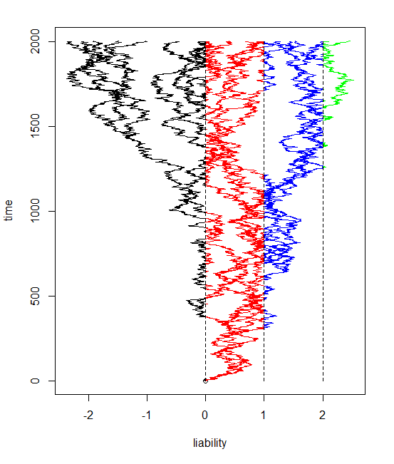
OK, first let's simulate a pure-birth phylogeny for (say) 200 species. We can also simulate our so-called liabilities up the tree with a correlation of 0.8:

> # load phytools & source
> library(phytools)
> source("threshBayes.R")
> # simulate
> tree<-pbtree(n=200,scale=1) # tree
> Xl<-sim.corrs(tree,vcv=matrix(c(1,0.8*sqrt(2),0.8*sqrt(2),2), 2,2)) # liabilities


Now, we can substitute one of these characters (say, trait 1) for a binary trait evolved under the threshold model, setting the threshold to +-0.

> X<-Xl
> X[Xl[,1]<0,1]<-0
> X[Xl[,1]>0,1]<-1
> X
     [,1]        [,2]
t1      0 -0.05615011
t2      1  0.42579821
t3      1 -0.32314924
t4      0  . . .


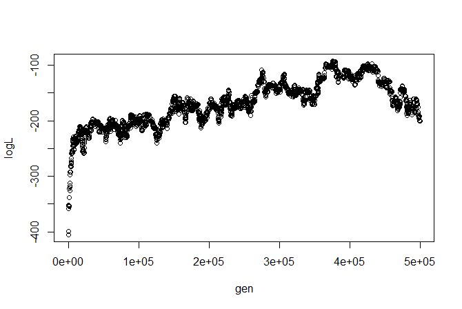
Now we are ready to run our MCMC. We'll just use the default control parameters and priors. Note that this may take some time - certainly at least several minutes even on a fast computer.

> mcmc<-threshBayes(tree,X,types=c("discrete","continuous"), ngen=500000)
[1] "gen 1000"
[1] "gen 2000"
[1] "gen 3000"
[1] . . .


The object returned by threshBayes is a list containing the posterior sample for the parameters of the evolutionary model and the liabilities at the tips. Note that for a continuous character liabilities are not sampled (they are treated as known), but these are still given in the posterior sample matrix. Also - we fix the rate of evolution at 1.0 for the liability of our discrete character. This is because don't actually have any information about the scale of our underlying liabilities, and the probability of switching back and forth between states on either side of the threshold is independent of the Brownian rate of evolution of liability (this is probably better explained in Felsenstein 2012).

We can, say, plot the likelihood profile:
I'm not sure how I feel about this likelihood profile (we might want to change our proposals or run multiple chains), but let's ignore these issues for illustrative purposes. (Remember, we can always run all the traditional MCMC diagnostics using, say, 'coda.')

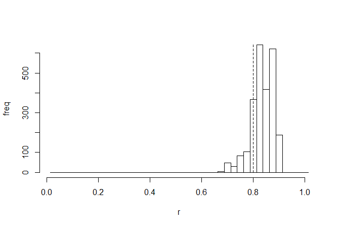
Let's cut off the first half of our posterior sample and get parameter estimates from the second 250,000 generations (2500 samples, in this case):

> estimates<-colMeans(mcmc$par[2501:nrow(mcmc$par),2:6])
> estimates
     sig1      sig2        a1        a2         r
1.0000000 2.0309112 0.6746904 1.1889742 0.8341032


These are really close to the generating parameters (particularly for σ2 and r). To be fair, this was part of my motivation in using a "large" tree of 200 taxa, even though run time is considerably longer. Parameter estimates from the posterior sample were not nearly as close on smaller trees.

We are probably most interested in the correlation coefficient - so let's look at the posterior sample for this parameter, with the generating value (0.8, in this case), overlain as a vertical dashed line:

> h<-hist(mcmc$par[2501:nrow(mcmc$par),"r"],0:40/40+0.0125, main=NULL,ylab="freq",xlab="r")
> lines(c(0.8,0.8),c(0,max(h$counts)),lty="dashed")


Finally, let's look at how close our true liabilities line up with estimates obtained by averaging the posterior sample:
> estLiab<-matrix(colMeans(mcmc$liab[2501:nrow(mcmc$liab), 1:200+1]),200,2)
> cor(Xl[,1],estLiab[,1])
[1] 0.9255481
> plot(Xl[,1],estLiab[,1],xlab="true liability",ylab="estimated liability")

Awesome. In this case, the generating & estimated liabilities match very well. Note that the estimated liabilities are scaleless - so although in this case they match well numerically, this is because we generated the liabilities under σ(liability)2=1.0. If we had instead simulated liabilities under a model of, say, σ(liability)2=100 or σ(liability)2=1000, then we would expect the correlation to be equivalent, but the liabilities themselves would not be as well matched numerically. Cool.

Next up - multiple states for the discrete character!

Bayesian MCMC for the threshold model

I'm going to write a shorter post about this than it deserves, but I have just programmed & posted a simple Bayesian MCMC version of the threshold model for discrete character evolution. This is the same model that is described by Felsenstein (2012) in his recent Am. Nat. paper.

In the quantitative genetic threshold model, we have a discretely valued characteristic that has an underlying quantitative basis, called liability. When the liability exceeds some threshold value, the trait changes state (say, from absence to presence or vice versa). The appeal of this model for analyzing discrete character evolution in the context of the tree is that it is (for many traits) more biologically realistic than a Markov-process model in which characters spontaneously turn on and off; and the probability of turning back on is independent of the time since "off." In addition, it allows us a framework for estimating the correlations between discrete and continuous characters, or between multiple discrete characters - this is just the correlation of their liabilities. For more about this model, I recommend the reference above.

Joe has already implemented a version of this model in his stand-alone program Threshml. There are some important differences between his implementation and my Bayesian version in R (threshBayes). These differences mean that parameter estimation will be highly similar, but not the same, between the two methods:

1. In Threshml, Joe uses MCMC to sample the liabilities for tip and internal nodes on the tree, and then computes the MLEs of the Brownian variances & covariances conditioned on the sampled liabilities. In my program, the liabilities, ancestral states at the root, correlation, and Brownian rates are sampled from their joint posterior probability distribution.

2. Because threshBayes is Bayesian, the user can control the prior probability distributions for the different parameters in the model. (Although if these are not supplied the program will try and compute sensible priors.)

3. The function threshBayes outputs the posterior sample, rather than a summary of the parameter estimates. This leaves more for the user to do, but it also means that the user can evaluate convergence & the like using MCMC diagnostics (such as those in the package 'coda').

4. Threshml runs multiple chains and combines the post burn-in results, whereas threshBayes only runs one chain. This doesn't seem to be that important, but if users want to run multiple chains they can do so manually, of course.

5. Threshml samples the liabilities at internal and tip nodes. threshBayes samples only the tip liabilities, and then computes their probability based on the sampled parameter values of the evolutionary model and root states on the tree.

6. Finally, as of now, Threshml can analyze an arbitrary number of characters; whereas threshBayes can only accept two traits (which can be any combination of discrete & continuous traits).

Check out the code for threshBayes on my phytools page. After lunch, I'll give an example simulation & result.

Thursday, August 16, 2012

Plotting error bars in two dimensions

This came up today in a conversation with a postdoc in my lab, Graham Reynolds.

There are probably more elegant ways to do this, but one simple solution for plotting error bars in two dimensions is provided by just calling the gplots function plotCI twice. Here's an example:

# simulate data
x<-rnorm(n=5,mean=4); y<-rnorm(n=5,mean=4)
# here is a completely arbitrary simulation model
# for the standard error/deviation
SDx<-runif(5,0.1,1); SDy<-runif(5,0.1,1)
# plot
# first get the limits for x & y +- error
xlim<-c(min(x-SDx),max(x+SDx))
ylim<-c(min(y-SDy),max(y+SDy))
# now plot twice, remember to set add=TRUE
plotCI(x,y,SDx,err="x",xlim=xlim,ylim=ylim)
plotCI(x,y,SDy,err="y",add=TRUE)


The result is not too bad:
There must be a function that automates this. If you know which one - please feel free to post it in "comments."

Tuesday, August 14, 2012

NESCent workshop & computer lab vignette

This past weekend I was a guest instructor in the NESCent Academy workshop entitled "Evolutionary Quantitative Genetics" that was co-organized by Joe Felsenstein & Steve Arnold. All the lectures from the course (including mine: 1, 2) are online - linked via the course website, above. In addition to lecturing, I also led a short computer lab in which I demonstrated some of the simulation, plotting, and comparative method capabilities of 'phytools'. Yesterday, I pulled all the lab material into an R vignette and the PDF is posted on the course website too (direct link to PDF). Check it out!

Thursday, August 9, 2012

Discrete time Brownian motion visualization

Working on my lecture for the Evolutionary Quantitative Genetics Workshop at NESCent. Here is some really simple code to perform discrete-time (non-phylogenetic) Brownian motion simulation:

# discrete time BM simulation
n<-100; t<-100; sig2<-1/t # set parameters
time<-0:t
X<-rbind(rep(0,n),matrix(rnorm(n*t,sd=sqrt(sig2)),t,n))
Y<-apply(X,2,cumsum)
plot(time,Y[,1],ylim=range(Y),xlab="time",ylab="phenotype", type="l")
apply(Y,2,lines,x=time)


And here is the result:

Wednesday, August 8, 2012

New version of phytools submitted to CRAN

I just submitted a new version of 'phytools' to CRAN (v0.1-9). I will be traveling to NESCent this Friday to participate in the Evolutionary Quantitative Genetics Workshop as a guest instructor. Since part of my guest instruction is a computer lab using phytools (and other R phylogenetics packages), hopefully this latest version will have been approved by CRAN and percolated through the mirrors by Saturday, the day of my lecture. In the interim, it is of course possible to download the source of this release from the phytools website. The image in the upper right-hand side of this post, by the away, is the icon for the so-called NESCent Academy, sponsor of the aforementioned workshop.

Some fixes in the functions from yesterday

This morning I fixed some bugs a couple of the new functions to phytools that I posted about yesterday: specifically fancyTree(...,type="traitgram3d") and phylomorphospace3d. I also made one minor change to anc.ML, my function for ancestral character estimation using maximum likelihood.

The most important updates were all to the function fancyTree. First, there was a problem in the way that I was passing optional arguments to and within the function using ... (dot-dot-dot or three dots). If one has a set of optional arguments, and you just want to pass them directly to another function that is going to be call internally, then this can be done using ... as a stand-in for these arguments. For instance:

foo<-function(x,y,...) plot(x,y,...)

will pass the optional arguments in ... directly to plot (which is a generic function with many optional arguments).

In my case, though, I wanted to gather optional arguments depending on a method (to be called internally), work with the arguments, and then send them to another function. I accomplished this (I believe correctly) using hasArg and list(...). This basically works as follows:

traitgram3d<-function(tree,...,control){
  if(hasArg(X)) X<-list(...)$X # get phenotypic data if provided
  else stop("no phenotypic data provided")
  if(!hasArg(A)){ # if ancestral states not provided
    ... # estimate ancestral states
  } else A<-list(...)$A # otherwise get them
  ... # do some other stuff
  phylomorphospace3d(tree,X,A,control=control) # plot
}


This seems to work, although it was somewhat difficult to find out online if this is the current best practice for optional arguments. Maybe a reader of the blog knows better!

As evidenced by the pseudocode above, fancyTree(...,type="traitgram3d") now accepts user supplied ancestral character states for internal nodes. We might have these, for instance, by simulation.

Finally, I also made some minor updates to phylomorphopsace3d (changing how the tip spheres are scaled) and anc.ML (adjusting the bound for optim(...,method="L-BFGS-B").

In addition to uploading these new function versions to the phytools page, I have also built a new package version (v 0.1-87) which can be downloaded here.

Tuesday, August 7, 2012

New nonstatic (i.e., non-CRAN) version of phytools, v0.1-86

I just posted a new version of phytools v0.1-86 to my website. You can download the source here and install as follows:

> install.packages("phytools_0.1-86.tar.gz",type="source", repos=NULL)

This version contains several new functions over the previous non-CRAN version v0.1-85 (fancyTree, phylomorphospace3d, and sim.corrs), as well as a longer list of new or updated functions from the last CRAN release (v0.1-8). I will probably work out a few more bugs, though, and submit this version (or something close to it) to CRAN this week.

Using phylomorphospace3d to plot 3D traitgrams

I realized after creating the three dimensional phylomorphospace function (phylomorphospace3d, described here) that one neat use of this function would be to do three dimensional traitgrams. That is, a projection of the tree into a space defined by time on one axis, and phenotype (in this case) on the other two.

This is relatively easy to do. This is because we've set up phylomorphospace3d to either estimate ancestral states or take them as input. To create a traitgram/phenogram - we just need to first estimate ancestral states for two characters, and then also compute the heights of internal and terminal nodes as our third "trait" (time from the root of the tree).

Both of these tasks are straightforward to accomplish. First, to estimate ancestral nodes for two characters encoded as columns in matrix X, we just do:

> require(phytools)
> A<-apply(X,2,function(x,tree) anc.ML(tree,x)$ace,tree=tree)


Then, we can compute the heights of internal and terminal nodes and attach them as columns in X and A, respectively.

> X<-cbind(X,diag(vcv(tree))[rownames(X)])
> A<-cbind(A,nodeHeights(tree)[match(rownames(A)[1:nrow(A)], tree$edge)])
> colnames(X)[3]<-colnames(A)[3]<-"time"


The final step, of course, just names our new trait axis what it is "time" since the root of the tree. With these parts, we can now use the new function phylomorphospace3d to plot our 3D traitgram.

I have built the steps above into the wrapper, fancyTree. To try it, just download the latest versions of the code for fancyTree (here) and phylomorphospace3d (here), load the source, and give it a try. The code below also uses the new simulation function sim.corrs, described here, but not yet a part of phytools.

> source("fancyTree.R")
> source("phylomorphospace3d.R")
> source("sim.corrs.R")
> require(phytools)
> tree<-pbtree(n=100,scale=10)
> X<-sim.corrs(tree,vcv=matrix(c(1,0.75,0.75,1),2,2))
> fancyTree(tree,type="traitgram3d",X)


And here's the result:


Cool.

New function to simulate multiple evolutionary correlations between characters in different parts of a tree

In phytools there are a couple of different functions based on my 2009 Evolution paper with Dave Collar for fitting multiple evolutionary correlations between characters to different parts of a phylogeny (Revell & Collar 2009). I just added a new function that can simulate multivariate evolution with arbitrarily different VCV matrices for the Brownian process for different states of a mapped discrete character (regimes) on the tree. To do this, I used a similar approach to the existing phytools function fastBM. In this case, however, I drew Brownian changes for multiple characters from their joint multivariate normal distributions. I did this separately for each mapped state; and then I added the changes along each edge together. The function (sim.corrs) is here.

We can test it out by generating under a multiple correlation model; and then fitting the model of Revell & Collar (2009) using evol.vcv. Let's try it out.

First, let's simulate a tree & character history using the functions pbtree and sim.history:

> tree<-sim.history(pbtree(n=100,scale=1), Q=matrix(c(-1,1,1,-1),2,2),anc=1)
> cols<-c("blue","red"); names(cols)<-c(1,2)
> plotSimmap(tree,cols,ftype="off",pts=F)


Next, load sim.corrs from source, create VCV matrices for simulation, and simulate:

> source("sim.corrs.R")
> vcv<-list(matrix(c(1,0.9,0.9,1),2,2), matrix(c(1,0.1,0.1,1.0),2,2))
> names(vcv)<-c(1,2)
> vcv
$`1`
     [,1] [,2]
[1,]  1.0  0.9
[2,]  0.9  1.0
$`2`
     [,1] [,2]
[1,]  1.0  0.1
[2,]  0.1  1.0
> X<-sim.corrs(tree,vcv)


Finally, let's fit our multiple VCV matrix model using evol.vcv. (We could also use evolvcv.lite to test a bunch of different models - including the common rates, different correlation model we used for simulation. More details here.)

> fit<-evol.vcv(tree,X)
> fit
$R.single
          [,1]      [,2]
[1,] 1.0603320 0.4342028
[2,] 0.4342028 0.8906066
$logL1
[1] -96.63233
$k1
[1] 5
$R.multiple
, , 1
          [,1]      [,2]
[1,] 0.9804452 0.8125698
[2,] 0.8125698 0.8371796
, , 2
          [,1]      [,2]
[1,] 1.1098840 0.1077934
[2,] 0.1077934 0.9188769
$logL.multiple
[1] -71.52816
$k2
[1] 8
$P.chisq
[1] 7.213247e-11
$convergence
[1] "Optimization has converged."


Cool. Both this and the other new functions will be in a new (& soon upcoming) version of phytools.

Updates to phylomorphospace3d

Yesterday I posted a new function phylomorphospace3d which uses the visualization package 'rgl' to project a tree into three dimensional morphospace (i.e., phylomorphospace). This morning I added some features to this function and posted an updated version here. Mainly these features add cosmetic improvement to the 3D plots; as well as allowing the user to control the plotting of axes, the box, and the font type. For instance, the following command was used to create the plot below in which I have simplified the axes and removed tip labels:

phylomorphospace3d(tree,X,control=list(ftype="off",simple.axes=T))

Monday, August 6, 2012

3D phylomorphospace plotting function

I just posted a preliminary version of a three-dimensional phylomorphospace function that uses the 3D visualization package 'rgl'. The visualization below is a video created using the function spin3d and movie3d. Phylomorphospace is just a projection of a phylogeny into (in this case) a three dimensional phenotype space. Leaves on the graph are the phenotypes of tip species. Lines connect tips to their common ancestors, reconstructed in morphospace using ML ancestral character estimation (phytools function anc.ML).


The function is relatively simple. I just create a set of matrices of dimensions equal to the matrix tree$edge. Then I fill the matrices using the values for tip species and the values for internal nodes. Next, I plot all the values for tip and internal nodes. I add the edges using the matrices described above. Finally, I plot tip labels - crudely adjusting them away from the tip vertices depending on the three dimensional position of the tip.

Source for the function is here. The function depends on 'rgl', not currently a dependency of phytools, so to run it do the following:

> install.packages("rgl")
> library(rgl)
> library(phytools)
> source("phylomorphospace3d.R")
> tree<-pbtree(n=10)
> X<-cbind(fastBM(tree),fastBM(tree),fastBM(tree))
> phylomorphospace(tree,X)

Friday, August 3, 2012

Plotting phylogenies with lineages leading to extinct taxa highlighted

I just created a new function, fancyTree, in which I intend to build in some custom wrappers to ape plot.phylo as well as phytools functions plotTree, plotSimmap, and phenogram to help phytools users draw special types of "fancy" phylogenetic trees.

I'm open to suggestions, of course, but my first idea was to create a function that would allow users to plot phylogenies containing extinct taxa (lineages terminating before the end of the tree) in a matter so as to highlight these branches. In particular, let's say we want to color branches of the tree leading either only to extinct taxa or proceeding in time the MRCA of all extant taxa in the tree a different color than the remaining branches (i.e, branches descended from the MRCA of all extant species and leading to extant species).

This should be pretty easy so long as we can identify all the branches that we want to color in this way. So let's think about how to do this. The first thing we need to do is identify the extant species and their common ancestor. We can do this using two functions in phytools, as follows:

extant<-getExtant(tree)
ca<-findMRCA(tree,extant)


Now, let's create a vector of all the edges in the tree (identified by the tipward node, i.e., the right column of tree$edge). We'll use this to keep score of which branches we want to flag:

edges<-rep(0,nrow(tree$edge))
names(edges)<-tree$edge[,2]


Now, after testing to see if the MRCA of extant species is the root node, and assuming that it is not, we can find all the edges preceding the MRCA of extant taxa using the phangorn function Descendants and the base function setdiff, as follows:

z<-setdiff(Descendants(tree,root.node,type="all"), Descendants(tree,ca,type="all"))
# now mark them in vector edges
edges[as.character(z)]<-1


Finally, we can go through the remaining nodes of the tree and determine if the descendants of each node above the MRCA of all extant taxa include extant taxa, both extant and extinct species, or only extinct species. In the final case, we should flag the branch in our vector edges. Here, we can just get a vector of all the nodes tipward of the MRCA; and then go through that vector and try to match the tips descended from each node in that vector to our vector of extant species, extant. This can be done as follows:

# get descendants of the MRCA
z<-Descendants(tree,ca,type="all")
# compute list of all descendants for each node in z
y<-Descendants(tree,z)
# finally, loop over y and flag edges not leaving
# extant descendants
for(i in 1:length(z))
   if(!any(tree$tip.label[y[[i]]]%in%extant))
      edges[as.character(z[i])]<-1


Note that there is some admittedly lazy programming above, because as soon as we visit an edge with no extant descendants, we should not visit any of its descendants, but we do anyway! This should be a simple thing to fix.

That's pretty much it. We can then use plot.phylo to create our tree, and voila!

plot.phylo(tree,edge.color=edges+1,edge.lty=edges+1,edge.width=2, no.margin=TRUE)


Code for this function can be downloaded from my phytools page and should be in the next version of the package.