Awesome new version of phenogram (in my opinion)

The phytools function phenogram does a projection of the phylogeny into a space defined by a morphological trait axis (on y) and time since the root (on x). This is a neat visualization, but it's most annoying attribute (in my opinion) is that the tip labels of taxa with similar phenotypes will often overlap in the plot, and can thus become unreadable or nearly so. Here's a quick example:

> require(phytools)
> tree<-pbtree(n=30)
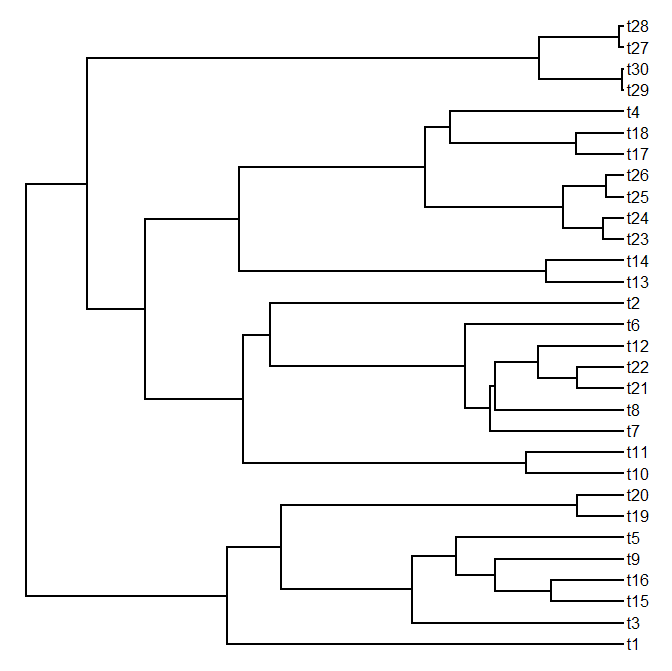
> plotTree(tree)

> x<-fastBM(tree)
> phenogram(tree,x)

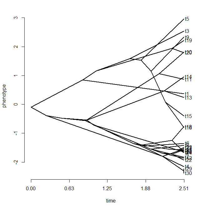
Wouldn't the plot above, you're probably thinking, look so much better if the taxon labels were spaced out somehow so that the tips could be more easily seen?

Well, this is now possible in the latest version of phenogram with the optional argument spread.labels=TRUE. This argument activates an internal function, spreadlabels, which uses numerical optimization to find that vertical label positions that simultaneously minimize the overlap between labels and the vertical distance from the position of the tip and the position of the label. The relative weight on each of these criteria (overlap & deviance, respectively) is controlled by the parameter spread.cost which is a vector that defaults to c(1,1), but can be adjusted by the user.

Ok, so the basic innovation is that we can spread out the tip labels now and retain a sensible plot. Let's try it with our plot from above:

> source("phenogram.R")
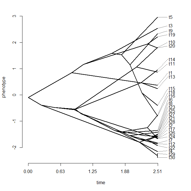
> phenogram(tree,x,spread.labels=TRUE,spread.cost=c(0.2,1))

This gives a much better spread of the tip labels than before, although in some case it's unclear (on parts of the phenotypic trait axis where species are clustered) which tip label matches with with tip.

This leads me to the other new feature of phenogram, which I'll explain by way of demonstration:

> phenogram(tree,x,spread.labels=TRUE,spread.cost=c(1,0.7), link=0.2,offset=0)

We can even push this to the extreme and space the tip labels out evenly on the trait axis, as follows:

> phenogram(tree,x,spread.labels=TRUE,spread.cost=c(1,0), link=0.2,offset=0)

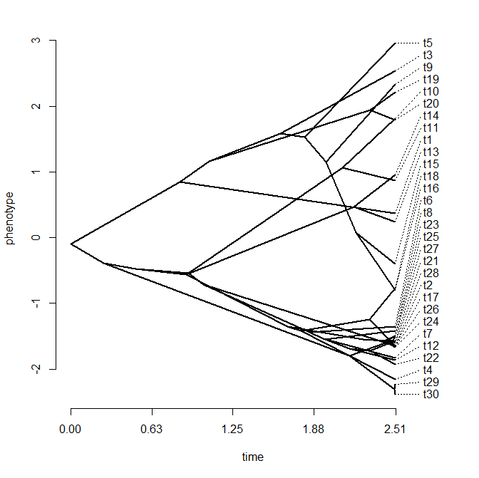
Pretty cool!

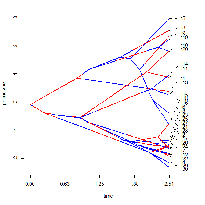
Finally, don't forget that phenogram can also be used to simultaneously plot a mapped discrete character on the tree. For instance:

> Q<-matrix(c(-1,1,1,-1),2,2)
> cols<-setNames(c("blue","red"),1:2)
> mtree<-sim.history(tree,Q)
> phenogram(mtree,x,colors=cols,spread.labels=TRUE, spread.cost=c(1,0.7),link=0.2,offset=0)

That's it!