There are a couple of different statistical methods that are commonly referred to as the phylogenetic ANOVA.
The phylogenetic ANOVA is generally meant to refer to the simulation approach of Garland et al. (
1993). Under this method, we fit the ANOVA model in the typical way - but then we conduct Brownian numerical simulations on the tree to obtain a null distribution of the model test statistic (
F). This Monte Carlo simulated null distribution is used for hypothesis testing. The Garland et al. (1993) phylogenetic ANOVA is implemented in the function
phy.anova from the geiger package, as well as in the phytools function
phylANOVA, which adds post-hoc tests.
The second approach is what I'm going to refer to as the phylogenetic
generalized least squares (GLS) ANOVA. Under this model we used the mechanics of GLS to fit a linear model in which the residual error of the model has phylogenetic autocorrelation. This is analogous, and mathematically equivalent, to fitting a phylogenetic regression (sensu Grafen
1989), as described in Rohlf (
2001).
The disadvantage of the former approach is that it cannot be used to estimate the coefficients of the fitted ANOVA model - only the p-value of this fit. This is because the OLS estimators (although statistically unbiased) are not minimum variance - and may have very high variance (probably depending on the phylogenetic structure of the independent variable). By contrast, GLS has the advantage of giving unbiased and minimum variance estimators of the fitted model coefficients - that is, conditioned on our model for the residual error being correct.
In spite of the similarity of the goals of these two different approaches, to my knowledge no prior study has compared their type I error or power. The code below can be used to estimate the type I error of each approach, as well as standard OLS (i.e., ignoring the phylogeny):
# load required packages
require(phytools)
require(nlme)
# number of replicates
N<-200
# balanced tree
tree<-compute.brlen(stree(n=128,type="balanced"))
# transition matrix for simulation
Q<-matrix(c(-2,1,1,1,-2,1,1,1,-2),3,3)
rownames(Q)<-colnames(Q)<-c(0,1,2)
# simulate discrete character
mtrees<-replicate(N,sim.history(tree,Q),simplify=FALSE)
class(mtrees)<-"multiPhylo"
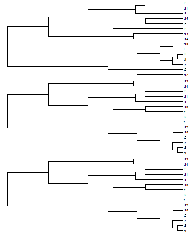
# plot (just for fun)
cols<-c("white","blue","red"); names(cols)<-0:2
foo<-function(x){
plotTree(x,ftype="off",lwd=5)
plotSimmap(x,cols,pts=FALSE,ftype="off",lwd=3,add=TRUE)
}
lapply(mtrees,foo)
# conduct simulations under the null
anovaOLS<-anovaPGLS<-anovaGarland<-list()
for(i in 1:N){
b<-c(0,0,0)
x1<-factor(mtrees[[i]]$states,levels=c(0,1,2))
e<-fastBM(mtrees[[i]])
y<-as.vector(b%*%t(model.matrix(~0+x1))+e)
anovaOLS[[i]]<-anova(gls(y~x1,data.frame(y,x1)))
anovaPGLS[[i]]<-anova(gls(y~x1,data.frame(y,x1), correlation=corBrownian(1,mtrees[[i]])))
anovaGarland[[i]]<-phylANOVA(mtrees[[i]],x1,y,posthoc=F)
print(paste("replicate",i))
}
# extract the p-values of the fitted models
pOLS<-sapply(anovaOLS,function(x) x$'p-value'[2])
pGLS<-sapply(anovaPGLS,function(x) x$'p-value'[2])
pGarland<-sapply(anovaGarland,function(x) x$Pf)
From here it is simple to get the type I error rate for each method:
> # get type I error
> typeI.OLS<-mean(pOLS<=0.05)
> typeI.GLS<-mean(pGLS<=0.05)
> typeI.Garland<-mean(pGarland<=0.05)
> typeI.OLS
[1] 0.85
> typeI.GLS
[1] 0.04
> typeI.Garland
[1] 0.06
So, it looks like Garland et al.'s simulation method and phylogenetic GLS both have appropriate type I error rates when there is no effect of the independent variable - but ignoring the phylogeny entirely can result in very high type I error. I should note that the simulation approach - using phylogenetic simulation of
x and Grafen's branch lengths - is kind of the "worst case scenario" for ignoring phylogeny.
We can loop around this code and ask whether the power to detect an effect of various sizes differs between PGLS-ANOVA and Garland et al.'s simulation approach. Here is the code I used as well as the result. To be able to run through this a little quicker, I decided to use only the first 100 trees from my prior simulation.
# power analysis
N<-100
power.GLS<-typeI.GLS; power.Garland<-typeI.Garland
anovaPGLS<-anovaGarland<-list()
for(i in 1:10){
for(j in 1:N){
# simulate an effect
# note that this relative to a variance between tips
# separated by the root of 1.0
b<-c(0,-0.1*i,0.1*i)
x1<-factor(mtrees[[j]]$states,levels=c(0,1,2))
e<-fastBM(mtrees[[j]])
y<-as.vector(b%*%t(model.matrix(~0+x1))+e)
anovaPGLS[[j]]<-anova(gls(y~x1,data.frame(y,x1), correlation=corBrownian(1,mtrees[[j]])))
anovaGarland[[j]]<-phylANOVA(mtrees[[j]],x1,y, posthoc=F)
print(paste("effect",i*0.1,"- replicate",j))
}
# extract the p-values of the fitted models
pGLS<-sapply(anovaPGLS,function(x) x$'p-value'[2])
pGarland<-sapply(anovaGarland,function(x) x$Pf)
# get power
power.GLS[i+1]<-mean(pGLS<=0.05)
power.Garland[i+1]<-mean(pGarland<=0.05)
}
plot(0:10/10,power.GLS,type="b",ylim=c(0,1), xlab="effect size",ylab="power")
lines(0:10/10,power.Garland,type="b")
lines(c(0,1),c(0.05,0.05),lty=2)
text(x=1,y=0.95,"PGLS",pos=2,offset=0)
text(x=1,y=0.7,"Garland et al.",pos=2,offset=0)

So, there you have it. If I've done this properly, it suggests that the Garland et al. simulation method has the correct type I error - but relatively low power compared to PGLS. Cool.
One caveat that I'd like to attach to all of this is that I've always found the presumed generating process - one in which the mean structure effectively evolves 'saltationally' (changing state spontaneously whenever the discrete character changes state) but the error structure evolves by Brownian evolution - to feel more than a little artificial.
That being said, I still feel that this result might interest some people. Could this be a published 'note?' I'm not sure, but feedback is welcome.