Adding vertical lines to a plotted tree

A user asks the following:

I want to plot vertical lines indicating various time points on my tree. . . . Is there an easy way to do this in R. . . ?

The answer turns out to be that yes - it is relatively easy to do this using the base function lines. Let's try:

First, let's use pbtree to simulate a tree and plot.phylo to plot it:

> tree<-pbtree(n=30,scale=100)
> x<-plot(tree)

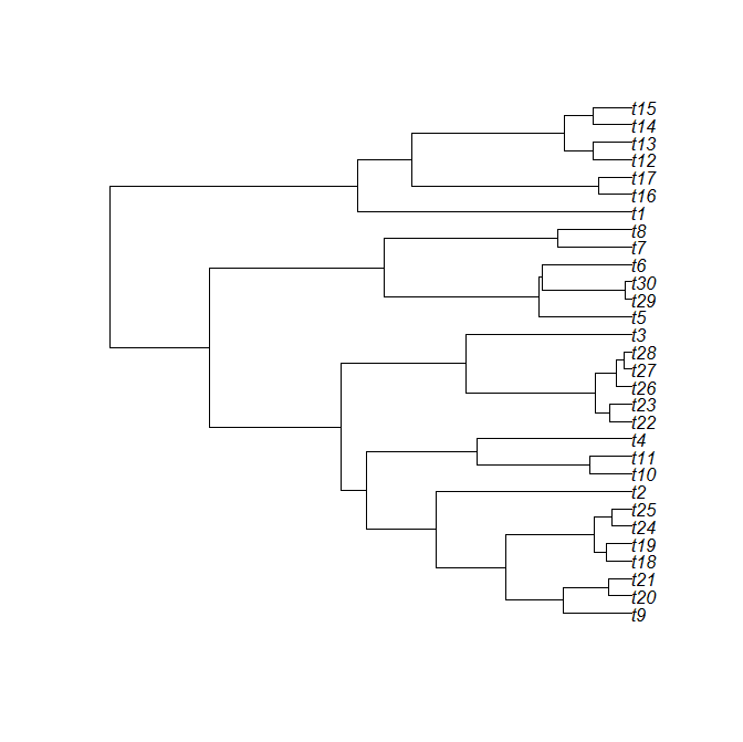
Ok, now, the dimensions of the plotted area in plot.phylo are 0 to the tree height (plus some extra space for the labels) on the horizontal axis; and 1 through the number of tips (here 30) on the vertical axis. In case we didn't know this already, it is also returned silently by plot.phylo. Here, we have stored this in x:

> x
$type
[1] "phylogram"
...
$x.lim
[1]   0.0000 108.3092
$y.lim
[1]  1 30
...
$Nnode
[1] 29

Now let's add lines at 25, 50, and 75 (time units) above the root:

> # with our plotting window still open
> lines(x=c(25,25),y=c(1,30),lwd=2)
> lines(x=c(50,50),y=c(1,30),lwd=2)
> lines(x=c(75,75),y=c(1,30),lwd=2)
> lines(x=c(75,75),y=c(-10,30),lwd=2)

(Note that all three lines are the same height - if they seem different that is an optical illusion!) Note that we can extend the lines a little bit beyond the dimensions given (say, in this case, using: lines(x=c(50,50),y=c(-10,40),lwd=2), for instance); however we cannot extend them to the edges of the plotting window unless we use: plot.phylo(...,no.margin=TRUE). Without the margin, what we did above would look as follows:

> x<-plot(tree,no.margin=TRUE)
> lines(x=c(25,25),y=c(-10,40),lwd=2)
> lines(x=c(50,50),y=c(-10,40),lwd=2)
> lines(x=c(75,75),y=c(-10,40),lwd=2)

We can do pretty much the same thing using phytools plotTree or plotSimmap, except that we need to keep in mind that these functions automatically rescale the horizontal plotting area (including labels) to unit length. To find the total height of the rescaled tree, we need to subtract the font size × the maximum string width of the tip labels from 1. So, in the case of plotSimmap, we would do:

> # simulate a character history
> tree<-sim.history(tree,Q=matrix(c(-1/20,1/20,1/20,-1/20),2,2))
> # set colors for plotting
> cols<-c("red","blue"); names(cols)<-c(1,2)
> # plot tree
> f<-1 # font size
> plotSimmap(tree,cols,pts=F,fsize=f)
> # add lines
> h<-1-f*max(strwidth(tree$tip.label))
> lines(x=c(0.25*h,0.25*h),y=c(-10,40),lwd=2)
> lines(x=c(0.5*h,0.5*h),y=c(-10,40),lwd=2)
> lines(x=c(0.75*h,0.75*h),y=c(-10,40),lwd=2)

Fot fun, let's combine this with make.era.map:

> tree<-make.era.map(tree,c(0,25,50,75,100))
> plotSimmap(tree,lwd=3,pts=F)
> h<-1-max(strwidth(tree$tip.label))
> lines(x=c(0.25*h,0.25*h),y=c(-10,40),lwd=3,col="red")
> lines(x=c(0.5*h,0.5*h),y=c(-10,40),lwd=3,col="green")
> lines(x=c(0.75*h,0.75*h),y=c(-10,40),lwd=3,col="blue")

Pretty cool.

New version of findMRCA for large trees

I just posted a new version of findMRCA that also works for very large trees. This is accomplished by using the new function (fastMRCA) that I posted earlier today. This function still calls nodeHeights, so for extremely large trees, it is still quite slow, but I it can still compute for up to at least 60,000 tips.

Just to reminder readers, findMRCA finds the MRCA of a list of species in a vector. It originally used the ape utility function mrca - but the problem with using that function is that it computes a n × n matrix of MRCAs for n species. This will be prohibitive for larger phylogenies.

The difference between the new and old versions of this function are even apparent even for relatively small trees. Let's try a tree with just 200 tips:

> require(phytools)
> tree<-rtree(n=200)
> system.time(a<-findMRCA(tree,c("t102","t112","t38","t145")))
   user  system elapsed 
   1.48    0.00    1.50 
> a
[1] 279
> source("findMRCA.R")
> system.time(b<-findMRCA(tree,c("t102","t112","t38","t145")))
   user  system elapsed 
   0.06    0.00    0.06 
> b
[1] 279

Direct link to the new function is here. I have also posted a new nonstatic version of phytools with the updated function. It can be downloaded from the following link and installed from source.

Function to efficiently return the MRCA of a pair of species for trees with many tips

A user reports that she wants to use the phytools function findMRCA to get the MRCA of a group of species. The problem is that her phylogeny is very large (~60,000 tips) and findMRCA uses the ape utility function mrca which does not work for very large trees. (The reason that mrca will not work for trees this large is probably because mrca returns a giant matrix containing the MRCA of every pair of species in the tree. For a tree with 60K taxa, this matrix would require over 14GB of memory.) She asks if there might be a different way to accomplish this task.

The way I approached this problem was first just to see if there was a more efficient way to get the MRCA of a single pair of species. There is. Here, I use the function Ancestors from the phangorn package:

fastMRCA<-function(tree,sp1,sp2){
    x<-match(sp1,tree$tip.label)
    y<-match(sp2,tree$tip.label)
    a<-Ancestors(tree,x)
    b<-Ancestors(tree,y)
    z<-a%in%b
    return(a[min(which(z))])
}

The code x<-match(sp1,tree$tip.label) translates the input tip name to a node number; a<-Ancestors(tree,x) returns a vector containing the node numbers of the ancestors of sp1, from the tip to the root; finally z<-a%in%b and a[min(which(z))] finds the elements of a that are in b, and then identifies which of these common elements are closest to the tips of the tree (i.e., the most recent). That's it! It seems to work, even on very large trees. The next natural step is use the same approach to find the MRCA of a set of species, just as in findMRCA.

New version of evolvcv.lite for multistate mapped trait

The existing phytools function evolvcv.lite fits the model of evol.vcv and Revell & Collar (2009), but with various constraints on the evolutionary rate matrices. Specifically, for two quantitative traits and a binary mapped character, evolvcv.lite fits the following four models: the same set of rates and single correlation for both states of the binary character (model 1 - this is the one rate matrix model in evol.vcv); different rates but the same correlation (model 2); different correlations but the same rates (model 3); and, finally, different correlations and rates (model 4 - this is the two rate matrix model from evol.vcv). The reason that I have not so far implemented these partially constrained models for more than two quantitative traits is because doing so constitutes a very challenging problem computationally. However there is no reason why the function could not be expanded to a mapped multistate character (rather than simply a binary character, as in the present implementation). In fact, a phytools user and blog reader recently requested this addition and I have finally gotten around to implementing and debugging this.

This version also fixes a bug in the previous edition which miscalculated the number of parameters (by -1 in all cases), and thus the AIC scores as well.

The new version of this function is here. I have also built a new version of phytools (here) which can be downloaded and installed from source.

One neat trick that I learned in the process of programming this update was how to add corresponding elements of list of matrices. Say, for instance, that X is a list of matrices of identical dimensions. It turns out that sumX<-Reduce("+",X) gives the sum of the matrices in X. Who knew!

Let's try out the new version of evolvcv.lite with an example.

> # install new version of phytools
> install.packages("phytools_0.1-82.tar.gz",type="source", repos=NULL)
Installing package(s) into ‘C:/R/win-library/2.14’
...
* DONE (phytools)
> require(phytools)
Loading required package: phytools
...
> # simulate tree & discrete character history
> tree<-sim.history(pbtree(n=100,scale=1), Q=matrix(c(-2,1,1,1,-2,1,1,1,-2),3,3))
> # simulate uncorrelated traits with three different rates
> # depending on the state
> X<-cbind(sim.rates(tree,c(1,2,3)),sim.rates(tree,c(1,2,3)))
> # fit models
> R<-evolvcv.lite(tree,X)
> # in the following I have hidden some results for brevity
> # only the full output for the best fitting model is shown
> R
$model1
$model1$description
[1] "common rates, common correlation"
...
$model1$AIC
[1] 379.6677

$model2
$model2$description
[1] "different rates, common correlation"
$model2$R
$model2$R$`1`
         [,1]     [,2]
[1,] 1.218973 0.096771
[2,] 0.096771 1.244826
$model2$R$`2`
         [,1]     [,2]
[1,] 1.6109460 0.1451599
[2,] 0.1451599 2.1194570
$model2$R$`3`
         [,1]     [,2]
[1,] 1.6255930 0.2015308
[2,] 0.2015308 4.0483984
$model2$logLik
[1] -181.8455
$model2$convergence
[1] 0
$model2$k
[1] 9
$model2$AIC
[1] 381.6911

$model3
$model3$description
[1] "common rates, different correlation"
...
$model3$AIC
[1] 382.892

$model4
$model4$description
[1] "no common structure"
...
$model4$AIC
[1] 385.1049

Cool. The best fitting model is our generating model in this case: common correlation but different rates depending on the state of our multistate character.

Addendum to previous post on plotting slanted phylograms with phytools::phenogram

In my last post I demonstrated how the phytools function phenogram could be used to plot a slanted phylogram - at least most of the time. The ape phylogenetics package function plot.phylo can also plot slanted phylograms (by setting type="cladogram" for a tree with branch lengths assigned), but this phylogram has a fundamentally different style than the type created by phenogram. The effect in particular is one in which the branches of the tree plotted with phenogram slant much more gently from the root than the branches in plot.phylo(...,type="cladogram"). The following graphic contrasts the two styles:

While I was musing about yesterday's post this morning, it occurred to me that plot.phylo(...,type="cladogram") kind of looks like it uses the same method as phenogram, but with the positions of the internal nodes determined by computing the "ancestral state" (that is, of the y coordinate of the tip) for the root node of each subtree separately. This could be accomplished using ace(...,method="pic") in the ape package. Well, this is not, in fact, how plot.phylo(...,type="cladogram") works, but the two methods visually present as almost identical. For instance:

> set.seed(1)
> tree<-read.tree(text=write.tree(pbtree(n=50)))
> plot.phylo(tree,type="cladogram")

> x<-1:50; names(x)<-tree$tip.label
> a<-ace(x,tree,method="pic")$ace
> x11(); phenogram(tree,c(x,a))

It turns out that both of these methods can sometimes result in lines that cross. For instance:

> set.seed(25)
> tree<-pbtree(n=50)
> plot.phylo(tree,type="cladogram")

Now, I'm not sure whether to characterize this as a bug in plot.phylo or not. Evidently, it is not always possible to avoid having lines cross when we want our tip labels to be evenly spaced on the vertical axis. This is stated in Felsenstein (2008; p. 576): "Note that with many of these methods (for plotting slanted phylograms), one cannot always avoid having lines cross. . . . The only way of avoiding crossing is to have the tips not be evenly spaced along the y axis." Clearly, in the above plotted example it would be possible to redraw this tree with the same horizontal branch lengths and no crossing lines, no?

Neat way to plot a slanted phylogram in phytools that almost always works

I'm not sure what I was doing when I thought to try this, but I realized that the phytools function phenogram can also be used to plot a neat looking slanted phylogram. This works as follows:

> tree<-pbtree(n=20,scale=100)
> # we do the following to make sure the tips are
> # in the right order
> tree<-read.tree(text=write.tree(tree))
> x<-1:length(tree$tip)
> names(x)<-tree$tip.label
> phenogram(tree,x)

Here the horizontal axis is time since the root, and the vertical axis doesn't mean anything of course. Unfortunately, as alluded in the post title, this only works most of the time - particularly when the tree has a lot of tips. For example, for one stochastic 50 taxon tree I get the following problem:

Obviously, the branches of the tree cross in a couple of different spots, which is no good. If we are determined to plot a tree in this format, we could try rotating the offending nodes above the problematic crossings and then replot our tree:

> plotTree(tree,node.numbers=T)

> tree<-rotate(tree,95)
> tree<-rotate(tree,53)
> tree<-read.tree(text=write.tree(tree))
> x<-1:length(tree$tip)
> names(x)<-tree$tip.label
> phenogram(tree,x)

It worked - at least for this particular case.

Some users might note that ape can also plot a slanted phylogram:

> plot.phylo(tree,type="cladogram")

But, obviously, this visualization has a very different look compared to the one we created previously. I'm not aware of other packages that might have an analogous function. Perhaps some readers of this blog are.

Painting different clades with different colors in phenogram function

A user recently submitted the following question:

is it possible to create a phenogram (that is, a projection of the tree into a two dimensional space defined by morphology on the vertical axis and time, see here) with different clades as different colors?

The function phenogram already allows a mapped discrete character, so if we want to color arbitrary clades on our tree different colors, we just need to combine phenogram with the phytools function paintSubTree, described here.

Let's try it in the following illustrating example:

> # first simulate a random tree
> tree<-pbtree(n=20,scale=100)
> # now plot the tree with node labels
> # so we can select the clades we want to paint
> plotTree(tree,pts=F,node.numbers=T)

OK, this tree has two main clades: one descended from node number "22", and the other descended from node number "26". Let's first paint the former clade with state "2" and the latter clade with state "3", we can leave the stem branches of each clade in state "1" (although we need not).

> tree<-paintSubTree(tree,node=22,state="2")
> tree<-paintSubTree(tree,node=26,state="3")
> # now let's plot using plotSimmap to ensure
> # that the correct branches were painted
> cols<-c("black","blue","red"); names(cols)<-1:3
> plotSimmap(tree,cols,pts=F,lwd=3,node.numbers=T)

Finally, let's simulate some data (normally, of course, we would read our data from file) and plot a traitgram using the phenogram function in phytools:

> x<-fastBM(tree)
> phenogram(tree,x,colors=cols,fsize=0.8)

That's it.