R trick 1: get the frequencies of factors in a vector

Here's a quick R hint. (I had briefly forgotten how to do this, and the solution wasn't totally obvious online.) Say I have a vector of factors in memory in R and I want to get the frequency or relative frequency of the different levels of the factor, I can do this using the base generic function summary. Just to see how this works, consider a vector containing the best-fitting quantitative trait evolution model for a set of 100 trees:

> best.fit
 [1] BM     BM     OU     lambda BM     BM     OU     BM
 [9] BM     BM     BM     lambda lambda BM     OU     BM
[17] BM     BM     OU     BM     BM     BM     lambda BM
[25] BM     BM     BM     OU     lambda BM     BM     BM
[33] BM     OU     BM     BM     lambda lambda lambda BM
[41] BM     BM     BM     OU     BM     BM     BM     BM
[49] BM     OU     BM     BM     BM     BM     BM     BM
[57] lambda lambda OU     OU     BM     BM     lambda BM
[65] BM     BM     BM     BM     lambda BM     BM     BM
[73] BM     OU     OU     BM     lambda BM     lambda BM
[81] BM     lambda BM     BM     BM     OU     BM     BM
[89] BM     BM     OU     OU     lambda BM     BM     BM
[97] BM     BM     OU     BM
Levels: BM lambda OU

We can count up the number or relative frequency of trees with each best fit model as follows:

> summary(best.fit)
   BM lambda     OU
   68     16     16
> summary(best.fit)/sum(summary(best.fit))
   BM lambda     OU
 0.68   0.16   0.16

That's it.

In the field

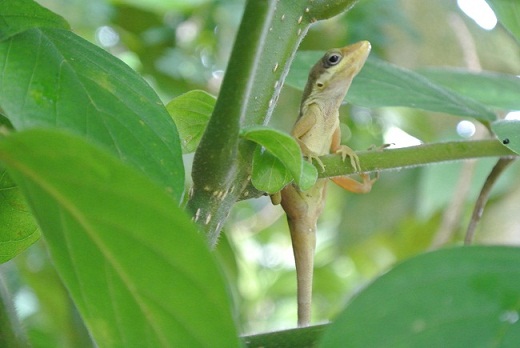
I'm presently in the field in Puerto Rico through June 26th, so I may not be blogging much on phytools; however I did post a short field story to Anole Annals (see link here) and I may do that a few more times before I'm done. BTW, the picture below is of Anolis krugi (the "mountain" grass-bush anole in Puerto Rico, although we are only at about 200 feet above sea level), one of the species we will be studying on the island.

New function to export data & trees in XML format for SIMMAP

Phytools has a function, make.simmap, that can be used to generate stochastic character mapped trees for discretely valued character data and phylogenies. This function, though, is really a much simplified version of Jonathan Bollback's stand alone program SIMMAP. The biggest difference between stochastic mapping in his program and with phytools::make.simmap is that my function first fits a model of character evolution using ML, and then samples from the conditional posterior distribution of character histories (conditioning on the fitted model), rather than the joint posterior distribution of substitution rates and character histories.

Some phytools users might therefore be interested in exporting their character data & trees for analysis in SIMMAP. In fact, I can attest to this because I want to do it - mainly to cross-validate a result that I obtained using make.simmap in phytools. Phytools can already be used to read in stochastic histories generated using SIMMAP (now both v1.0 and v1.5).

SIMMAP (v1.5, I'll get to v1.0 later) reads trees and data in XML format. XML is a markup language, like HTML, using tags for different components of the data structure. SIMMAP can read both DNA and discrete, numerically coded morphological traits. The former is called datatype="nucleotide" by SIMMAP and the latter datatype="standard" by SIMMAP.

I have now posted a function online, export.as.xml, that can create an XML datafile using data stored in various formats and a tree or multiple trees stored as a "phylo" or "multiPhylo" object (respectively).

A direct link to the code is here. I will also most likely include it in future releases of phytools. (I may also include the capacity to export for SIMMAP v1.0. SIMMAP v1.0 does not use XML, but a modified NEXUS format, and is still in fairly wide use.)

Blomberg's K (phylogenetic signal) with intraspecific variability, more than one sample per species, error in the estimation of species means, etc.

I feel certain that I have addressed this in several past posts, but due to some recent R-sig-phylo and phytools user inquiries, I thought I would just re-post a general procedure for computing phylogenetic signal with intraspecific variability. This includes estimation of signal with multiple observations per species, and computing phylogenetic signal when species means are uncertain. I start by assuming that the data are a vector x in which species names are in names(x) (and thus observations from the same species have the same names). I assume also that the tree (a "phylo" object) is contained in tree.

A little aside might be worthwhile to mention here. When we read in our data from file, we often have our species names in the first column of the input file. We would then do (say) X<-read.table(...,row.names=1) so that R will use the first column of our input data file as the row names of the data table, X. The problem with this in the case of multiple observations per species is that the data type "data.frame" does not allow row names to repeat. In this case, we should just read the row names in in the first column of X, and then do: x<-X[,2]; names(x)<-X[,1], which will give us what we want.

To incorporate estimation error (i.e., multiple observations per species) we should use the method of Ives et al. (2007). To do this, we need sampling errors for each species. This presents a problem when we have a data set that consists of multiple observations for some species - but only one per species for others. In this situation, I recommend assuming that the variances we cannot calculate (i.e., the ones for species with only one observation) are equal to the mean within-species variance. We could also use a pooled within species variance, putting more weight on the variances calculated for species with large sample sizes. Either assumption will be safest if the intraspecific variance is not too heterogeneous among species, and if we have log-transformed our data before analysis. Neither procedure is all that difficult (the pooled variance calculation is just a touch trickier), so I will demonstrate both.

> require(phytools)
> # first let's simulate a tree & data for the purposes
> # of demonstration (normally read from file)
> N<-300 # number of species for simulation
> tree<-pbtree(n=N)
> # simulate the true species means
> xhat<-fastBM(tree)
> phylosig(tree,xhat)
[1] 0.9623659
> # simulate 1-20 observations per species
> # with the same intraspecific variance
> x<-sampleFrom(xhat,rep(1,N),randn=c(1,20))
> # get the means by species
> temp<-aggregate(x,by=list(names(x)),mean)
> xbar<-temp[,2]; names(xbar)<-temp[,1]
> # get the variance by species
> temp<-aggregate(x,by=list(names(x)),var)
> xvar<-temp[,2]; names(xvar)<-temp[,1]
> # get the sample size per species
> n<-as.vector(table(names(x)))
> # replace NA with mean (m) or pooled (p) variance
> xvarm<-xvarp<-xvar
> xvarm[is.na(xvar)]<-mean(xvar,na.rm=TRUE)
> xvarp[is.na(xvar)]<-0
> xvarp[is.na(xvar)]<-
   sum((n-1)*xvarp/(sum(n[n>1])-length(n[n>1])))
> # compute K ignoring sampling error
> phylosig(tree,xbar)
[1] 0.6166613
> # compute K with sampling error, mean variance for n=1
> phylosig(tree,xbar,se=sqrt(xvarm/n))
$K
[1] 0.9476694
$sig2
[1] 1.039297
$logL
[1] -444.4693
> # compute K with sampling error, pooled variance for n=1
> phylosig(tree,xbar,se=sqrt(xvarp/n))
$K
[1] 0.947966
$sig2
[1] 1.039077
$logL
[1] -444.4875

One characteristic feature that emerges from this is that phylogenetic signal is underestimated (here fairly dramatically, although this will depend on the amount of sampling error we've ignored) when uncertainty in the estimation of species means is ignored. This is a general phenomenon. We do much better when we include it in our estimating procedure.

Adding vertical lines to a plotted tree

A user asks the following:

I want to plot vertical lines indicating various time points on my tree. . . . Is there an easy way to do this in R. . . ?

The answer turns out to be that yes - it is relatively easy to do this using the base function lines. Let's try:

First, let's use pbtree to simulate a tree and plot.phylo to plot it:

> tree<-pbtree(n=30,scale=100)
> x<-plot(tree)

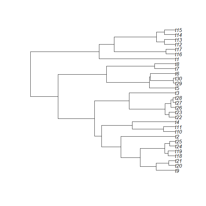Ok, now, the dimensions of the plotted area in plot.phylo are 0 to the tree height (plus some extra space for the labels) on the horizontal axis; and 1 through the number of tips (here 30) on the vertical axis. In case we didn't know this already, it is also returned silently by plot.phylo. Here, we have stored this in x:

> x
$type
[1] "phylogram"
...
$x.lim
[1]   0.0000 108.3092
$y.lim
[1]  1 30
...
$Nnode
[1] 29

Now let's add lines at 25, 50, and 75 (time units) above the root:

> # with our plotting window still open
> lines(x=c(25,25),y=c(1,30),lwd=2)
> lines(x=c(50,50),y=c(1,30),lwd=2)
> lines(x=c(75,75),y=c(1,30),lwd=2)
> lines(x=c(75,75),y=c(-10,30),lwd=2)

(Note that all three lines are the same height - if they seem different that is an optical illusion!) Note that we can extend the lines a little bit beyond the dimensions given (say, in this case, using: lines(x=c(50,50),y=c(-10,40),lwd=2), for instance); however we cannot extend them to the edges of the plotting window unless we use: plot.phylo(...,no.margin=TRUE). Without the margin, what we did above would look as follows:

> x<-plot(tree,no.margin=TRUE)
> lines(x=c(25,25),y=c(-10,40),lwd=2)
> lines(x=c(50,50),y=c(-10,40),lwd=2)
> lines(x=c(75,75),y=c(-10,40),lwd=2)

We can do pretty much the same thing using phytools plotTree or plotSimmap, except that we need to keep in mind that these functions automatically rescale the horizontal plotting area (including labels) to unit length. To find the total height of the rescaled tree, we need to subtract the font size × the maximum string width of the tip labels from 1. So, in the case of plotSimmap, we would do:

> # simulate a character history
> tree<-sim.history(tree,Q=matrix(c(-1/20,1/20,1/20,-1/20),2,2))
> # set colors for plotting
> cols<-c("red","blue"); names(cols)<-c(1,2)
> # plot tree
> f<-1 # font size
> plotSimmap(tree,cols,pts=F,fsize=f)
> # add lines
> h<-1-f*max(strwidth(tree$tip.label))
> lines(x=c(0.25*h,0.25*h),y=c(-10,40),lwd=2)
> lines(x=c(0.5*h,0.5*h),y=c(-10,40),lwd=2)
> lines(x=c(0.75*h,0.75*h),y=c(-10,40),lwd=2)

Fot fun, let's combine this with make.era.map:

> tree<-make.era.map(tree,c(0,25,50,75,100))
> plotSimmap(tree,lwd=3,pts=F)
> h<-1-max(strwidth(tree$tip.label))
> lines(x=c(0.25*h,0.25*h),y=c(-10,40),lwd=3,col="red")
> lines(x=c(0.5*h,0.5*h),y=c(-10,40),lwd=3,col="green")
> lines(x=c(0.75*h,0.75*h),y=c(-10,40),lwd=3,col="blue")

Pretty cool.

New version of findMRCA for large trees

I just posted a new version of findMRCA that also works for very large trees. This is accomplished by using the new function (fastMRCA) that I posted earlier today. This function still calls nodeHeights, so for extremely large trees, it is still quite slow, but I it can still compute for up to at least 60,000 tips.

Just to reminder readers, findMRCA finds the MRCA of a list of species in a vector. It originally used the ape utility function mrca - but the problem with using that function is that it computes a n × n matrix of MRCAs for n species. This will be prohibitive for larger phylogenies.

The difference between the new and old versions of this function are even apparent even for relatively small trees. Let's try a tree with just 200 tips:

> require(phytools)
> tree<-rtree(n=200)
> system.time(a<-findMRCA(tree,c("t102","t112","t38","t145")))
   user  system elapsed 
   1.48    0.00    1.50 
> a
[1] 279
> source("findMRCA.R")
> system.time(b<-findMRCA(tree,c("t102","t112","t38","t145")))
   user  system elapsed 
   0.06    0.00    0.06 
> b
[1] 279

Direct link to the new function is here. I have also posted a new nonstatic version of phytools with the updated function. It can be downloaded from the following link and installed from source.

Function to efficiently return the MRCA of a pair of species for trees with many tips

A user reports that she wants to use the phytools function findMRCA to get the MRCA of a group of species. The problem is that her phylogeny is very large (~60,000 tips) and findMRCA uses the ape utility function mrca which does not work for very large trees. (The reason that mrca will not work for trees this large is probably because mrca returns a giant matrix containing the MRCA of every pair of species in the tree. For a tree with 60K taxa, this matrix would require over 14GB of memory.) She asks if there might be a different way to accomplish this task.

The way I approached this problem was first just to see if there was a more efficient way to get the MRCA of a single pair of species. There is. Here, I use the function Ancestors from the phangorn package:

fastMRCA<-function(tree,sp1,sp2){
    x<-match(sp1,tree$tip.label)
    y<-match(sp2,tree$tip.label)
    a<-Ancestors(tree,x)
    b<-Ancestors(tree,y)
    z<-a%in%b
    return(a[min(which(z))])
}

The code x<-match(sp1,tree$tip.label) translates the input tip name to a node number; a<-Ancestors(tree,x) returns a vector containing the node numbers of the ancestors of sp1, from the tip to the root; finally z<-a%in%b and a[min(which(z))] finds the elements of a that are in b, and then identifies which of these common elements are closest to the tips of the tree (i.e., the most recent). That's it! It seems to work, even on very large trees. The next natural step is use the same approach to find the MRCA of a set of species, just as in findMRCA.