New version of densityMap

The full title of this post should read New much faster version of densityMap that returns the plotted map invisibly combined with generic plotting method for special mapping object class, or something like that - but that seemed like a tongue twister. densityMap is a function to visualize the posterior sample of maps from a stochastic mapping analysis and is described in an article that I have in press at Methods in Ecology & Evolution.

I just posted a new version of densityMap (code here) that simultaneously addresses a couple of significant issues with this (otherwise pretty cool, in my opinion) function.

Firstly, prior versions of the function are way too slow. The function is still slow - just no longer way too slow. This speed-up was achieved entirely using the trick of removing the class attribute of our "multiPhylo" object which - for some reason that is not entirely clear to me - dramatically speeds up handling of the object both by apply family functions, and even in for loops.

Secondly, what makes densityMap especially annoying to work with - given that it is slow - is that to alter any of the plotting options, you need to re-compute the aggregate mappings. In the new version of densityMap (and new minor phytools build, phytools 0.2-60), densityMap plots the mapped tree as before, but also returns a special object of class "densityMap" invisibly. This can then be plotted using a call of the generic plot (to which I have added the phytools method plot.densityMap).

Here's a demo:

> require(phytools)
Loading required package: phytools
> packageVersion("phytools")
[1] ‘0.2.60’
> # simulate tree & data
> tree<-pbtree(n=70,scale=1)
> Q<-matrix(c(-1,1,1,-1),2,2)
> rownames(Q)<-colnames(Q)<-c(0,1)
> tree<-sim.history(tree,Q)
> x<-tree$states
> # generate stochastic maps
> mtrees<-make.simmap(tree,x,nsim=100)
make.simmap is sampling character histories conditioned on the transition matrix
Q =
          0          1
0 -0.8857354  0.8857354
1  0.8857354 -0.8857354
(estimated using likelihood);
and (mean) root node prior probabilities
pi =
  0  1
0.5 0.5
Done.
> # generate density map
> # this would have been much slower before
> system.time(map<-densityMap(mtrees))
sorry - this might take a while; please be patient
  user  system elapsed
  7.85    0.12    7.97

Now, in earlier versions of densityMap if we wanted to adjust the way this plot looked (say - so that the labels don't overlap!) - we would have to recompute the aggregate mapping (which, remember, took us 8s here - but much longer in earlier versions or for bigger trees). However, here we have created the object maps, which we can then pass to plot.densityMap with our revised plotting options:

> plot(map,lwd=5,fsize=c(0.7,1),legend=0.4)

for example.

Cool.

Issue with plotting output trees from SIMMAP using densityMap

A phytools user contacted me yesterday with the following issue:

I was trying to use your densityMap function to visualize some output from SIMMAP. The mutational mappings seemed to work fine in SIMMAP. I tried importing into R using read.simmap, this seemed to work fine. I then tried to use densityMap but it keeps giving me the following error:
> trees<-read.simmap(file)
> densityMap(trees,res=1000)
sorry - this might take a while; please be patient
Error in lower:upper: NA/NaN argument

This isn't something that I'd seen before, but I recognized that the code is from a part of the function in which the beginning and ending points for each map segment on a branch (XX) is compared to a matrix containing the beginning and ending points for every step interval along the same edge (YY); in which these steps are based on the edge length of the branch and the function argument res. Importantly, the beginnings and endings are in terms of the height above the root.

This made me suspect that the problem was with the edge lengths of the tree. densityMap assumes that the topology of the input trees are equal with proportional branch lengths. (In fact, there is an option - densityMap(...,check=TRUE) - that evaluates this equality criterion, and returns an error message if it fails.) For some reason that I don't completely understand (and even when 'mutational mapping' is performed on a single input tree), SIMMAP returns a sample of trees with varying total length. Theoretically, this should not be a problem if the branch lengths are strictly proportional. Unfortunately, due to numerical precision (which is relatively low - 6 digit - in the SIMMAP output), the branch lengths of these varyingly scaled trees are not strictly proportional. Consequently, even after they have been scaled to the same total length using phytools function rescaleSimmap (which is done internally in densityMap), the trees have slightly different branch lengths - sufficiently different, evidently, to account for this error.

My eventual workaround was to write a function that would apply one set of branch lengths (say, from a reference tree) to another tree or set of trees. For basic "phylo" objects, this is trivial of course. We would just do:

# for reference tree tr1
tr2$edge.length<-tr1$edge.length

However, for trees with mappings, it is slightly more complicated. Here is a simplified version of the function:

applyBranchLengths<-function(tree,edge.length){
  if(class(tree)=="multiPhylo"){
    trees<-lapply(tree,applyBranchLengths,
      edge.length=edge.length)
    class(trees)<-"multiPhylo"
    return(trees)
  } else {
    tree$edge.length<-edge.length
    if(!is.null(tree$maps)){
      for(i in 1:nrow(tree$edge)){
        temp<-tree$maps[[i]]/sum(tree$maps[[i]])
        tree$maps[[i]]<-temp*tree$edge.length[i]
      }
    }
    return(tree)
  }
}

This function uses the proportional time spent in each state along each edge of the target tree in rescaling the mappings to the reference tree. (I've left out calculation of the $mapped.edge matrix here, which involves a few more lines of code.) I have posted the full function code for this here.

Anyway, it worked! Here's a quick demo with a simulated tree & dataset in which I performed stochastic mapping using SIMMAP v1.5 for another project:

> trees<-read.simmap("simmap.trees.nex",format="nexus", version=1.5)
> densityMap(trees)
sorry - this might take a while; please be patient
Error in lower:upper : NA/NaN argument
> # get the tree heights
> h<-sapply(trees,function(x) max(nodeHeights(x)))
> h
 [1] 13.215321  6.213479 16.864350  9.936482 ....
 ...
> # ok, they have different heights - is that the problem?
> # try rescaling
> rescaled<-rescaleSimmap(trees,mean(h))
> densityMap(rescaled)
sorry - this might take a while; please be patient
Error in lower:upper : NA/NaN argument
> # nope!
> # ok, how about *not* rescaling, but applying the
> # relative branch lengths from trees[[1]] to all the
> # trees in the sample
> newbl<-mapply(applyBranchLengths,trees, lapply(as.list(h),"*",trees[[1]]$edge.length/h[1]), SIMPLIFY=FALSE)
> class(newbl)<-"multiPhylo"
> # these trees have their original total lengths
> # but relative branch lengths from trees[[1]]
> densityMap(newbl,fsize=c(0.6,1))
sorry - this might take a while; please be patient

densityMap with non-binary trait data

I (not-so) recently go the following question about the phytools function densityMap:

Is it possible to make same as your method 1 'Visualizing the aggregate result of stochastic mapping, in your paper (2013) : “Two new graphical methods for mapping trait evolution on phylogenies”, for a discrete trait which is not a binary trait?

Presently densityMap, which creates a visualization of the posterior probability density from stochastic mapping of a binary character on the tree, does not work for any more than two characters. This is mostly because it is hard to envision visualizing color in more than one dimension! (One possibly for a three-state character would be to put the probabilities on a 3D RGB scale - but this adds only one dimension to the analysis anyway.)

The only solution right now is to use mergeMappedStates on the "simmap" trees & then plot "A" vs. "not A", "B" vs. "not B", "C" vs. "not C", etc.

Here is a quick demo of how to do that, which would have to be varied depending on the specific character states that were being modeled:

library(phytools)
packageVersion("phytools")

## [1] '0.4.99'

## simulate some data
Q<-matrix(c(-1,0.5,0.5,
    0.5,-1,0.5,
    0.5,0.5,-1),3,3)
rownames(Q)<-colnames(Q)<-LETTERS[1:3]
## true history
tree<-sim.history(pbtree(n=50,scale=1),Q,anc="A")

## Done simulation(s).

tree

## 
## Phylogenetic tree with 50 tips and 49 internal nodes.
## 
## Tip labels:
##  t32, t33, t23, t13, t14, t7, ...
## 
## The tree includes a mapped, 3-state discrete character with states:
##  A, B, C
## 
## Rooted; includes branch lengths.

plot(tree,fsize=0.8)

## no colors provided. using the following legend:
##        A        B        C 
##  "black"    "red" "green3"

## simulated tip data
x<-getStates(tree,"tips")

trees<-make.simmap(tree,x,nsim=100,model="ER")

## make.simmap is sampling character histories conditioned on the transition matrix
## Q =

##            A          B          C
## A -0.8584049  0.4292025  0.4292025
## B  0.4292025 -0.8584049  0.4292025
## C  0.4292025  0.4292025 -0.8584049

## (estimated using likelihood);
## and (mean) root node prior probabilities
## pi =

##         A         B         C 
## 0.3333333 0.3333333 0.3333333

## Done.

trees

## 100 phylogenetic trees with mapped discrete characters

print(trees[1:10],details=TRUE)

## 10 phylogenetic trees with mapped discrete characters
## tree 1 : 50 tips, 3 mapped states
## tree 2 : 50 tips, 3 mapped states
## tree 3 : 50 tips, 3 mapped states
## tree 4 : 50 tips, 3 mapped states
## tree 5 : 50 tips, 3 mapped states
## tree 6 : 50 tips, 3 mapped states
## tree 7 : 50 tips, 3 mapped states
## tree 8 : 50 tips, 3 mapped states
## tree 9 : 50 tips, 3 mapped states
## tree 10 : 50 tips, 3 mapped states

## merge B & C
tBC<-lapply(trees,mergeMappedStates,c("B","C"),"B or C")
class(tBC)<-c("multiSimmap","multiPhylo")
print(tBC[1:10],details=TRUE)

## 10 phylogenetic trees with mapped discrete characters
## tree 1 : 50 tips, 2 mapped states
## tree 2 : 50 tips, 2 mapped states
## tree 3 : 50 tips, 2 mapped states
## tree 4 : 50 tips, 2 mapped states
## tree 5 : 50 tips, 2 mapped states
## tree 6 : 50 tips, 2 mapped states
## tree 7 : 50 tips, 2 mapped states
## tree 8 : 50 tips, 2 mapped states
## tree 9 : 50 tips, 2 mapped states
## tree 10 : 50 tips, 2 mapped states

obj<-densityMap(tBC,plot=FALSE,states=c("B or C","A"))

## sorry - this might take a while; please be patient

obj

## Object of class "densityMap" containing:
## 
## (1) A phylogenetic tree with 50 tips and 49 internal nodes.
## 
## (2) The mapped posterior density of a discrete binary character with states (B or C, A).

plot(obj,outline=TRUE,lwd=4,fsize=c(0.7,1))

Providing the argument states=c("B or C","A") is an important undocumented detail here, because otherwise branches of high posterior probability would be high posterior probability of "B or C"!

Similarly:

tAC<-lapply(trees,mergeMappedStates,c("A","C"),"A or C")
class(tAC)<-c("multiSimmap","multiPhylo")
obj<-densityMap(tAC,plot=FALSE,states=c("A or C","B"))

## sorry - this might take a while; please be patient

obj

## Object of class "densityMap" containing:
## 
## (1) A phylogenetic tree with 50 tips and 49 internal nodes.
## 
## (2) The mapped posterior density of a discrete binary character with states (A or C, B).

plot(obj,outline=TRUE,lwd=4,fsize=c(0.7,1))

tAB<-lapply(trees,mergeMappedStates,c("A","B"),"A or B")
class(tAB)<-c("multiSimmap","multiPhylo")
obj<-densityMap(tAB,plot=FALSE,states=c("A or B","C"))

## sorry - this might take a while; please be patient

obj

## Object of class "densityMap" containing:
## 
## (1) A phylogenetic tree with 50 tips and 49 internal nodes.
## 
## (2) The mapped posterior density of a discrete binary character with states (A or B, C).

plot(obj,outline=TRUE,lwd=4,fsize=c(0.7,1))

Thanks for the question!

Circular trees in densityMap and contMap

In an earlier post I showed how plotSimmap(...,type="fan") could be used to plot densityMap or contMap style plots using the object of class "densityMap" or "contMap" returned invisibly by each function, respectively.

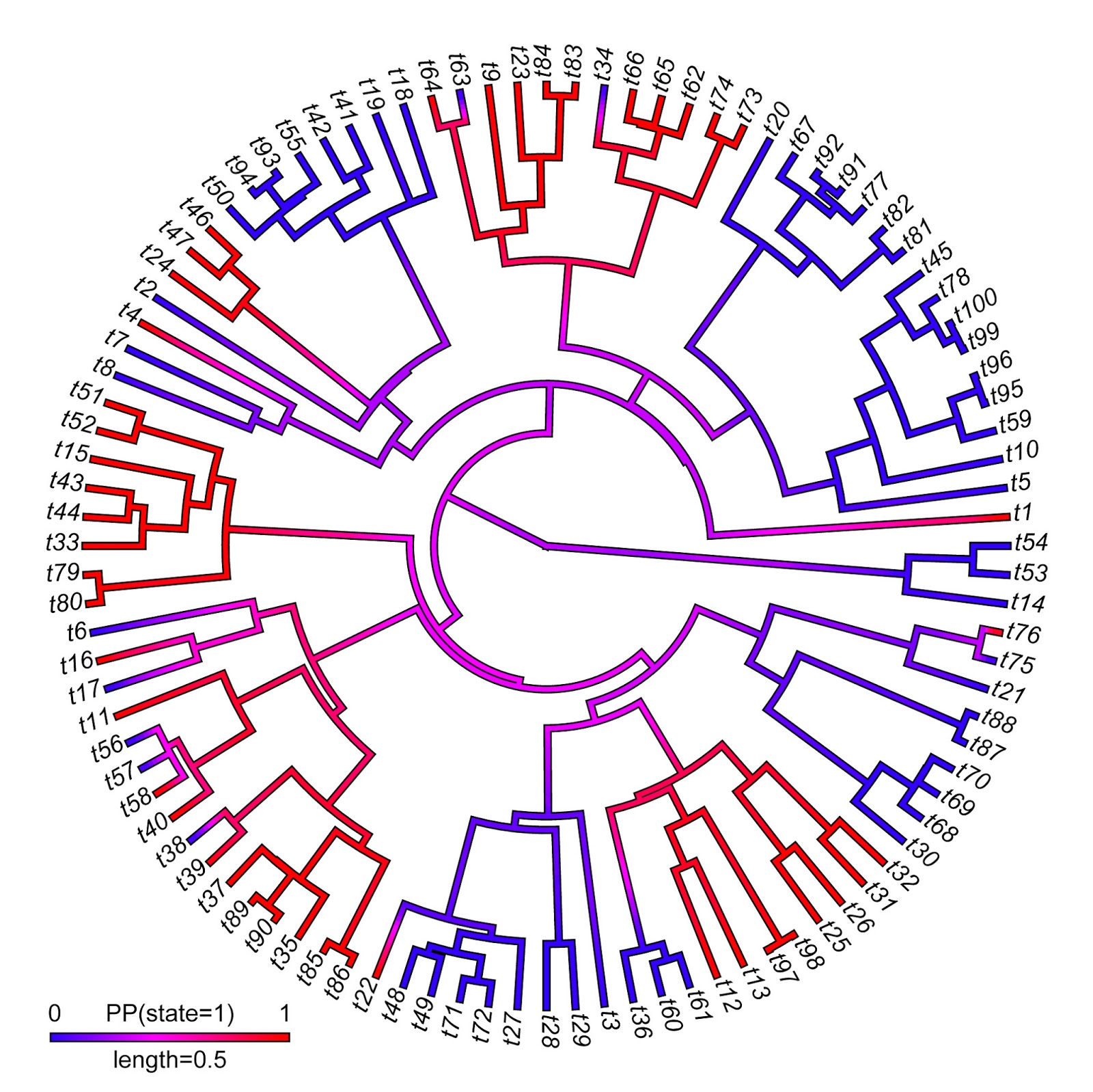
Well, I have now build this directly into contMap & densityMap (and the S3 generic plot for objects of class "densityMap" and "contMap"). Check it out:

> require(phytools)
Loading required package: phytools
> packageVersion("phytools")
[1] ‘0.2.76’
> contMap(tree,x,type="fan",fsize=0.9)

> X<-densityMap(mtrees,outline=TRUE,fsize=0.9)
sorry - this might take a while; please be patient

Argh - way too cluttered. Let's try a circular tree instead!

> class(X)
[1] "densityMap"
> plot(X,type="fan",fsize=0.9,outline=TRUE)

Since these updates involved changes to a number of methods in phytools - the best bet is to update to the latest non-CRAN phytools build (phytools 0.2-76).

That's it.

Update to densityMap, new minor phytools version

I just posted a new version of the function to plot the posterior density of a binary character mapped on the tree using stochastic character mapping (described here). The updated code is on the webpage for phytools, but if you want to use this function version, you are probably better off updating to the most recent, minor release of phytools, v0.2-04, here. This is because I also had to make some changes to the phytools functions plotTree, plotSimmap, and densityMap, so doing a package update from source is the best way to ensure that you have the correct versions of each function installed.

The biggest difference between this version of densityMap and the previous one is that in this version more control of how the plot looks has been migrated to the user. In particular, the user can control the width of plotted edges as well as whether or not to display a fine black outline around the lines of the tree graph. These may seem like minor changes, but to plot the outline I first use plotTree to plot a tree with lwd+2 width edges. Then I overlay the densityMap tree. To do this, I had to modify plotTree (which is actually just a wrapper for plotSimmap) so that it could be used to plot multiple trees in the same plotting object. In addition, in previous versions of plotSimmap, the offset of tip labels is a function of the plotted edge widths. This meant that when I plotted to trees in the same object, but with different width edges, the tip labels did not overlay exactly. The way I fixed this is by migrating control of the label offset to the function arguments - and then I used a label offset based only on the interior, densityMap line widths.

Here's an example of the result:

> # install package
> install.packages("phytools_0.2-04.tar.gz",type="source", repos=NULL)
** installing *source* package 'phytools' ...
...
* DONE (phytools)
> library(phytools)
Loading required package: ape
Loading required package: mnormt
...
> # simulate random Yule tree
> tree<-pbtree(n=50,scale=2)
> # simulate data on the tree using sim.history
> Q<-matrix(c(-2,2,2,-2),2,2,dimnames=list(c(0,1),c(0,1)))
> tree<-sim.history(tree,Q)
> # generating stochastic map trees (500, in this case)
> trees<-make.simmap(tree,tree$states,nsim=500)
> # create density map
> densityMap(trees,fsize=c(1,1),outline=TRUE,lwd=6, res=1000)
sorry - this might take a while; please be patient
>

Note that this is pretty slow - to make it quicker, use fewer maps (say 100) or a lower "resolution" (densityMap argument res), which is just the number of times the probability/color is sampled along any path from the root to the tips.

Bug fix in drop.tip.densityMap

A phytools user reported the following peculiar bug with the phytools function drop.tip.densityMap:

## simulate some data
library(phytools)
tree<-pbtree(n=26,tip.label=LETTERS,scale=1)
Q<-matrix(c(-1,1,1,-1),2,2,dimnames=list(letters[1:2],letters[1:2]))
x<-as.factor(sim.history(tree,Q)$states)

## Done simulation(s).

x

## A B C D E F G H I J K L M N O P Q R S T U V W X Y Z 
## b b b a a b a b b b b b a a a a b a a b b b a a a b 
## Levels: a b

## now replicate the error
trees<-make.simmap(tree,x,nsim=100)

## make.simmap is sampling character histories conditioned on the transition matrix
## Q =

##           a         b
## a -3.440867  3.440867
## b  3.440867 -3.440867

## (estimated using likelihood);
## and (mean) root node prior probabilities
## pi =

##   a   b 
## 0.5 0.5

## Done.

obj<-densityMap(trees,plot=FALSE)

## sorry - this might take a while; please be patient

plot(obj,lwd=4,outline=TRUE)

tips<-sample(tree$tip.label,5)
tips

## [1] "I" "U" "N" "G" "V"

obj<-drop.tip.densityMap(obj,tips)

## x should be an object of class "contMap"

I'm not sure when I introduced this bug, but it is now fixed and this will be in the next version of phytools (or if you update phytools from GitHub).

obj<-densityMap(trees,plot=FALSE)

## sorry - this might take a while; please be patient

source("../phytools/R/densityMap.R")
obj<-drop.tip.densityMap(obj,tips)
plot(obj,lwd=4,outline=TRUE)

That's it.