Showing posterior probabilities from describe.simmap at the nodes of a plotted tree

A user comment asks the following:

"I wonder how can I alter the size of the "pie" in describe.simmap.... Same question for altering the color...."

Well, there is no way at present to change the color or pie-size in describe.simmap(...,plot=TRUE); however, describe.simmap, it is easy to recreate the posterior probability plot of describe.simmap using the function output - while customizing its attributes.

Here's a quick demo:

> # check package version
> packageVersion("phytools")
[1] ‘0.2.54’
>
> # first simulate some data to use in the demo
> Q<-matrix(c(-2,1,1,1,-2,1,1,1,-2),3,3)
> rownames(Q)<-colnames(Q)<-letters[1:3]
> tree<-sim.history(pbtree(n=50,scale=1),Q)
> x<-tree$states
>
> # now the demo
> mtrees<-make.simmap(tree,x,model="ER",nsim=100)
make.simmap is sampling character histories conditioned on the transition matrix
Q =
          a        b        c
a -2.041867  1.020934  1.020934
b  1.020934 -2.041867  1.020934
c  1.020934  1.020934 -2.041867
(estimated using likelihood);
and (mean) root node prior probabilities
pi =
        a        b        c
0.3333333 0.3333333 0.3333333
Done.
> XX<-describe.simmap(mtrees,plot=FALSE)
100 trees with a mapped discrete character with states:
a, b, c

trees have 23.93 changes between states on average

changes are of the following types:
      a,b  a,c  b,a  b,c  c,a  c,b
x->y 2.11 2.91 4.62 5.77 4.94 3.58

mean total time spent in each state is:
            a        b        c    total
raw  2.2816521 4.1930936 4.2593925 10.73414
prop 0.2125603 0.3906316 0.3968081  1.00000

> hh<-max(nodeHeights(tree))*0.02 # for label offset
> plot(tree,no.margin=TRUE,label.offset=hh,edge.width=2)
> nodelabels(pie=XX$ace,piecol=c("blue","red","green"), cex=0.5)
> tiplabels(pie=to.matrix(x,colnames(XX$ace)), piecol=c("blue","red","green"),cex=0.5)

Obviously, to adjust the pie-sizes & colors we just change the values of cex & piecol.

That's it.

New article describing new graphical methods: densityMap, contMap, and fancyTree(...,type="phenogram95")

My new article describing three new graphical methods for plotting comparative data on trees, implemented in the phytools functions densityMap (1, 2, 3, 4), contMap (1, 2, 3), and fancyTree(..., type="phenogram95") just came out "Accepted" (i.e., manuscript pages, not type-set or proofed) in Methods in Ecology & Evolution. The article is entitled Two new graphical methods for mapping trait evolution on phylogenies, which might seem like a bit of a misnomer (or perhaps a tribute to this article) given my description, above, but I think it makes sense.

The figure at right is from the paper (click for a larger version with tip labels). Thanks to Dave Collar for helpfully providing the published data & tree.

2x faster version of make.simmap for Q="mcmc"

In a previous post I promised that I could speed up make.simmap(..., Q="mcmc"), i.e., the full Bayesian MCMC make.simmap method. (Matt Pennell said he didn't care, which is very generous of him.)

There was one really low-hanging fruit which is that during Bayesian MCMC sampling of the transition matrix, Q, make.simmap was unnecessarily computing the likelihood twice for each iteration of the MCMC. This is because make.simmap uses modified code from ape's ace function internally to perform Felsenstein's pruning algorithm in computing the likelihood of Q as well as well as the conditional scaled likelihoods at each node. Normally, ace returns the likelihood & the scaled conditional likelihoods of the subtrees at each internal node by first maximizing the likelihood using the optimizer nlminb, and the computing the conditional likelihoods given MLE(Q). I modified the code to take a fixed value of Q, however it still returned both the overall log-likelihood & the conditional likelihoods via two rounds of the pruning algorithm. For the vast majority of generations in our MCMC we don't care about the conditional scaled likelihoods (because we're not sampling that generation) so we should only compute the overall log-likelihood which we need to compute the posterior odds ratio and make a decision about whether to retain the updated parameter values or not. Whenever we want to sample a particular value for Q (i.e., every samplefreq generations), we can compute the conditional likelihoods for all the nodes - since we'll need these later.

This improvement has a pretty dramatic effect on computation time - pretty much halving it as you might expect. Here's a demo using my not-too-fast i5 desktop:

> # simulate tree & data
> Q<-matrix(c(-1,1,1,-1),2,2)
> colnames(Q)<-rownames(Q)<-LETTERS[1:2]
> tree<-sim.history(pbtree(n=100,scale=1),Q)
> x<-tree$states
> # number of changes, etc., on the true tree
> describe.simmap(tree)
1 tree with a mapped discrete character with states:
 A, B

tree has 21 changes between states

changes are of the following types:
  A  B
A  0 11
B 10  0

mean total time spent in each state is:
              A          B    total
raw  11.5075650 10.5967548 22.10432
prop  0.5206025  0.4793975  1.00000

> # OK, now let's run make.simmap & time it
> system.time(mtrees.old<-make.simmap(tree,x,Q="mcmc", nsim=200,prior=list(beta=2,use.empirical=TRUE)))
Running MCMC burn-in. Please wait....
Running 20000 generations of MCMC, sampling every 100 generations. Please wait....
make.simmap is simulating with a sample of Q from the posterior distribution
Mean Q from the posterior is
Q =
          A        B
A -1.205146  1.205146
B  1.205146 -1.205146
and (mean) root node prior probabilities
pi =
[1] 0.5 0.5
Done.
  user  system elapsed
398.44    0.23  401.99
> # pretty slow!!
> describe.simmap(mtrees.old)
200 trees with a mapped discrete character with states:
 A, B

trees have 29.93 changes between states on average

changes are of the following types:
        A,B    B,A
x->y 15.055 14.875

mean total time spent in each state is:
              A          B    total
raw  11.3629822 10.7413376 22.10432
prop  0.5140616  0.4859384  1.00000

OK - now let's compare to the updated version:

> source("make.simmap.R")
> system.time(mtrees.new<-make.simmap(tree,x,Q="mcmc", nsim=200,prior=list(beta=2,use.empirical=TRUE)))
Running MCMC burn-in. Please wait....
Running 20000 generations of MCMC, sampling every 100 generations. Please wait....
make.simmap is simulating with a sample of Q from the posterior distribution
Mean Q from the posterior is
Q =
          A        B
A -1.227405  1.227405
B  1.227405 -1.227405
and (mean) root node prior probabilities
pi =
[1] 0.5 0.5
Done.
  user  system elapsed
214.87    0.03  216.36
> # still slow, but better
> describe.simmap(mtrees.new)
200 trees with a mapped discrete character with states:
 A, B

trees have 29.975 changes between states on average

changes are of the following types:
        A,B  B,A
x->y 14.585 15.39

mean total time spent in each state is:
              A          B    total
raw  11.1900994 10.9142203 22.10432
prop  0.5062404  0.4937596  1.00000

The code for this version is here, but I have also posted a new phytools build (phytools 0.2-54). Check it out & please report any issues or bugs.

Stochastic mapping with a bad informative prior results in parsimony reconstruction

The title to this post pretty much says it all. As alluded to in the discussion thread of an earlier post, if you use an informative prior probability distribution in which the mean is too low - then the result can (especially in the limiting case as the mean goes to zero) become the parsimony reconstruction. That is, as our prior probability distribution forces our posterior distribution of Q to be closer & closer to zero, all reconstructions converge to the one or multiple most parsimonious reconstructions.

Here's a quick demonstration of what I mean. Just to make the point clear, I have used a very exaggerated bad prior probability density - the γ with α = 2 & β = 200 - which basically says we have a high degree of confidence that the rate of evolution is very low (with mean α/β = 0.01).

> library(phytools)
Attaching package: ‘phytools’

> # first create a mapped history
> Q<-matrix(c(-2,2,2,-2),2,2)
> colnames(Q)<-rownames(Q)<-LETTERS[1:2]
> tree<-sim.history(pbtree(n=100,scale=1),Q,anc="A")
> describe.simmap(tree)
1 tree with a mapped discrete character with states:
A, B

tree has 54 changes between states

changes are of the following types:
   A  B
A  0 18
B 36  0

mean total time spent in each state is:
             A         B    total
raw  12.897944 15.049629 27.94757
prop  0.461505  0.538495  1.00000

> x<-tree$states
> # now let's perform stochastic mapping with a
> # reasonable prior
> emp.prior<-make.simmap(tree,x,nsim=100,Q="mcmc", prior=list(beta=2,use.empirical=TRUE))
Running MCMC burn-in. Please wait....
Running 10000 generations of MCMC, sampling every 100 generations. Please wait....
make.simmap is simulating with a sample of Q from the posterior distribution
Mean Q from the posterior is
Q =
          A        B
A -1.943666  1.943666
B  1.943666 -1.943666
and (mean) root node prior probabilities
pi =
[1] 0.5 0.5
Done.

> # now a prior that is way too low!
> low.prior<-make.simmap(tree,x,nsim=100,Q="mcmc", prior=list(alpha=2,beta=200))
Running MCMC burn-in. Please wait....
Running 10000 generations of MCMC, sampling every 100 generations. Please wait....
make.simmap is simulating with a sample of Q from the posterior distribution
Mean Q from the posterior is
Q =
          A          B
A -0.1103515  0.1103515
B  0.1103515 -0.1103515
and (mean) root node prior probabilities
pi =
[1] 0.5 0.5
Done.

> # plot all three for comparison to the true tree
> layout(matrix(c(1,2,3),1,3))
> plotSimmap(tree,pts=F,lwd=2,ftype="off")
no colors provided. using the following legend:
      A      B
"black"  "red"
> plotSimmap(emp.prior[[1]],pts=F,lwd=2,ftype="off")
...
> plotSimmap(low.prior[[1]],pts=F,lwd=2,ftype="off")
...

What's dangerous about the reconstructions shown above is that (without the known true history, as in this case) it may be the rightmost reconstruction - the one obtained with the faulty prior - that looks most reasonable!

OK - let's do a little more analysis to further the point:

> describe.simmap(emp.prior)
100 trees with a mapped discrete character with states:
A, B

trees have 60.09 changes between states on average

changes are of the following types:
      A,B  B,A
x->y 29.52 30.57

mean total time spent in each state is:
              A          B    total
raw  15.7298487 12.2177248 27.94757
prop  0.5628341  0.4371659  1.00000

> describe.simmap(low.prior)
100 trees with a mapped discrete character with states:
A, B

trees have 22.97 changes between states on average

changes are of the following types:
      A,B  B,A
x->y 14.44 8.53

mean total time spent in each state is:
              A          B    total
raw  17.7439790 10.2035945 27.94757
prop  0.6349023  0.3650977  1.00000

> # get parsimony score
> library(phangorn)
> X<-phyDat(as.matrix(x),type="USER",levels=LETTERS[1:2])
> parsimony(tree,X)
[1] 22

Of course, we can push it even further & virtually guarantee that our stochastic maps have the MP number of changes, e.g.:

> really.low.prior<-make.simmap(tree,x,nsim=20,Q="mcmc", prior=list(alpha=1,beta=1e4))
Running MCMC burn-in. Please wait....
Running 2000 generations of MCMC, sampling every 100 generations. Please wait....
make.simmap is simulating with a sample of Q from the posterior distribution
Mean Q from the posterior is
Q =
            A            B
A -0.002198051  0.002198051
B  0.002198051 -0.002198051
and (mean) root node prior probabilities
pi =
[1] 0.5 0.5
Done.
> describe.simmap(really.low.prior)
20 trees with a mapped discrete character with states:
A, B

trees have 22.05 changes between states on average

changes are of the following types:
      A,B B,A
x->y 13.65 8.4

mean total time spent in each state is:
              A          B    total
raw  17.4916200 10.4559534 27.94757
prop  0.6258726  0.3741274  1.00000

Well, you get the idea.

Method comparison in make.simmap

A couple of days ago I introduced a new version of make.simmap that uses Bayesian MCMC to sample the transition matrix, Q, from its posterior probability distribution rather than fixing it at the MLE (as in previous versions of the function). The idea is that by fixing Q we are ignoring variation in the reconstructed evolutionary process that is due to uncertainty in the transition matrix.

I thought that, as a first pass, it might be neat to compare these two approaches: one in which we fix Q at its most likely value; and the other in which Q is sampled from its posterior probability distribution. My expectation is relatively straightforward - variance on estimated variables should go up (hopefully towards their true variance), and the probability that the generating parameter values should be on their corresponding (1-α)% CIs (which, in general, included less than (1-α)% of generating values in the empirical Bayes method) should go to (1-α).

My analysis was as follows:

1. First, I simulated 200 pure-birth trees containing 100 taxa using the phytools function pbtree. On each tree I simulated the stochastic history of a binary discrete character with two states (a & b) given a symmetric transition matrix with backward & forward rate Q_a,b = Q_b,a = 1.0.

2. For each tree, I computed the number of transitions of each type and of any type; and the fraction of time spent in state a vs. b.

3. Next, for each tree I sampled 200 stochastic character maps conditioning on the MLE transition matrix (Q="empirical").

4. For each set of stochastic maps, I computed the number and type of transitions as well as the time spent in state a and averaged them across maps. I also obtained 95% credible intervals on each variable from the sample of stochastic maps, in which the 95% CI is the interval defined by the 2.5th to 97.5th percentiles of the sample. I calculated the total fraction of datasets in which the true values fell on the 95% CI from stochastic mapping.

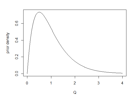
5. Finally, I repeated 1. through 4. but this time stochastic maps were obtained by first sampling 200 values of Q from its Bayesian posterior distribution using MCMC (Q="mcmc"). In this case, I used 1,000 generations of burn-in followed by 20,000 generations of MCMC, sampling every 100 generations. I used a γ prior probability distribution with make.simmap(...,prior(use.empirical=TRUE, beta=2)), which means that the parameters of the prior distribution were β = 2 and α = MLE(Q) × β. The figure below shows the γ prior probability density for α = β = 2.

Here are some of the results. First let's look at the empirical Bayes method in which Q is set to its most likely value:

> ci<-colMeans(on95); ci
   a,b    b,a      N time.a
 0.895  0.925  0.800  0.970
> pbinom(ci*200,200,0.95)
       a,b        b,a          N     time.a
0.00115991 0.07813442 0.00000000 0.93765750

This shows that - although the method is not too bad, the 95% CI coverage is significantly below the nominal level - at least for the number of changes from a to b as well as the total number of changes on the tree.

Now let's see a visual summary of the results across simulations:

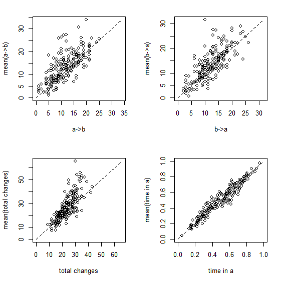
Figure 1

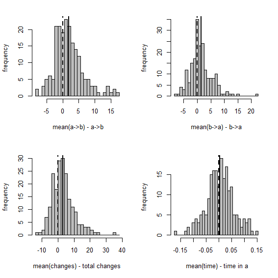
Figure 2

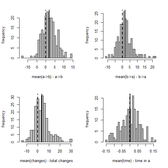
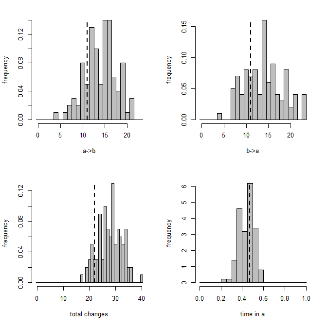
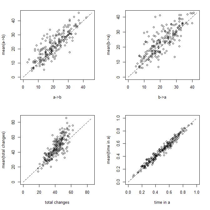
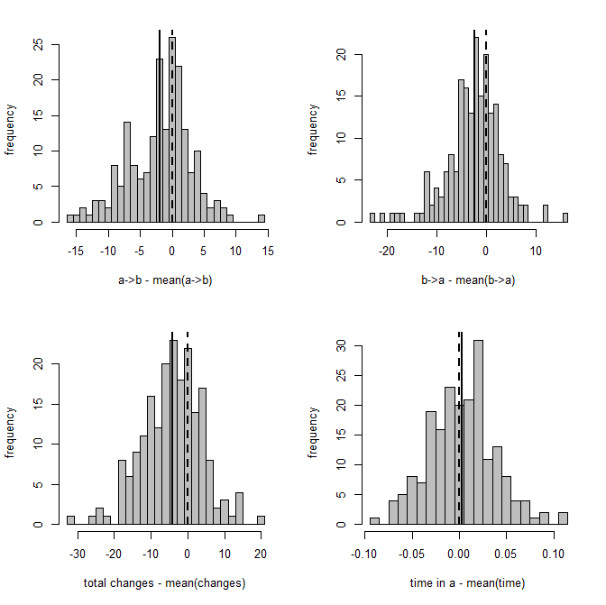
Figure 1 shows a set of scatterplots with the true & estimated values of each of the four variables described earlier. Figure 2 is just a different visualization of the same data - here, though, we have the frequency distribution, from 200 stochastic maps, of the difference between the estimated and generating values.

OK, now let's compare to the full* Bayesian version in which MCMC is used to sample Q from its posterior probability distribution.

(*Note that in a true fully Bayesian method I should not have used my empirical data to parameterize the prior distribution, which I have done here by using prior=list(...,use.empirical=TRUE), but let's ignore that for the time being.)

First, the 95% CI, as before:

> ci<-colMeans(on95); ci
   a,b    b,a      N time.a
 0.970  0.925  0.955  0.940
> pbinom(ci*200,200,0.95)
       a,b        b,a          N     time.a
0.93765750 0.07813442 0.67297554 0.30024430

Neat. This time our (1-α)% CIs include the true values of our 4 variables about (1-α)% of the time; and in no case is this significantly lower than we'd expect by chance.

Here are the same two visualizations as for the empirical Bayes method, above:

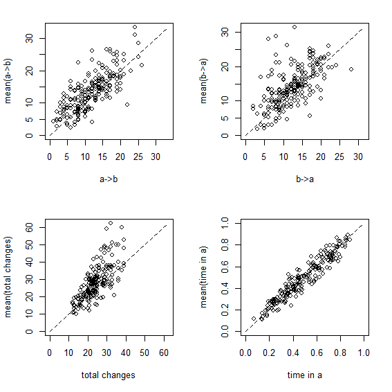
Figure 3

Figure 4

Overall, this shows us that integrating over uncertainty in Q - at least in this simple case - does have the desired effect of expanding our (1-α)% credible interval to include the generating values of our variables in (1-α)% of simulations. Cool.

Unfortunately, make.simmap(...,Q="mcmc") is very slow. I have some ideas about a few simple ways to speed it up and I will work on these things soon.

New test "full" version of make.simmap

I just posted a new version of make.simmap that samples stochastic histories not only conditioned on the most likely value of Q, but that can also use a fixed value of Q, or can sample Q from its posterior probability distribution conditioned on the substitution model. Pretty cool!

The motivation underlying this is that prior versions of make.simmap sampled stochastic histories by fixing Q. This is empirical Bayesian because we are fixing one level of the model - in this case, the transition matrix - at its most likely value given the data, rather than sampling from the posterior distribution. This should be unbiased - but it will cause the variance on estimated parameters to be too low. We can see this in the simulation I posted recently - although the effect is small when the tree & tip data contain lots of information about the evolutionary transition rates. By fixing Q we circumvent the (perhaps) challenging tasks of specifying prior densities.

Well, this empirical Bayes method remains available as an option in make.simmap (in fact, as the default - because I think it makes sense for most users) - but now users can also sample Q, rather than merely assuming a fixed value. The way this works is as follows:

1. For each tree, we obtain nsim samples from the posterior distribution by nsim × samplefreq generations of MCMC (after burnin). We also keep the conditional likelihoods from the pruning algorithm from each value of Q in this step.

2. For each value of Q & set of conditional likelihoods, we simulate a set of node states and stochastic map up the tree.

make.simmap uses a γ prior probability distribution for the rates with α & β that can be specified by the user. By default, α = β = 1.0, but this will probably not be a good prior density for your dataset.

make.simmap also offers the option of allowing the data to inform the prior distribution. This is accomplished using make.simmap(...,prior= list(use.empirical=TRUE)). In this case, only β from the specified γ distribution will be used - and α will be set at α = β × ML(Q).

Let's experiment with the function:

> packageVersion("phytools")
[1] ‘0.2.53’
> require(phytools)
Loading required package: phytools
> # simulate data & tree > Q<-matrix(c(-1,1,1,-1),2,2)
> rownames(Q)<-colnames(Q)<-letters[1:2]
> tree<-pbtree(n=100,scale=1)
> tree<-sim.history(tree,Q)
> x<-tree$states
> # describe.simmap on true history
> AA<-describe.simmap(tree,message=FALSE)
> # perform stochastic mappings using the empirical
> # priors method
> mtrees<-make.simmap(tree,tree$states,nsim=100, model="ER",Q="mcmc",prior=list(beta=3,use.empirical=TRUE))
Running MCMC burn-in. Please wait....
Running 10000 generations of MCMC, sampling every 100 generations. Please wait....
make.simmap is simulating with a sample of Q from the posterior distribution
Mean Q from the posterior is
Q =
         a         b
a -1.009082  1.009082
b  1.009082 -1.009082
and (mean) root node prior probabilities
pi =
[1] 0.5 0.5
Done.
> # describe.simmap on stochastic maps
> XX<-describe.simmap(mtrees,message=FALSE)

Here's a summary of the results:

Now let's compare to the empirical Bayes method in which we fix Q at its most likely value:

> mtrees<-make.simmap(tree,x,nsim=100,model="ER", Q="empirical")
make.simmap is sampling character histories conditioned on the transition matrix
Q =
           a          b
a -0.9704866  0.9704866
b  0.9704866 -0.9704866
(estimated using likelihood);
and (mean) root node prior probabilities
pi =
 a   b
0.5 0.5
Done.
> # describe.simmap on stochastic maps
> YY<-describe.simmap(mtrees,message=FALSE)

Some results:

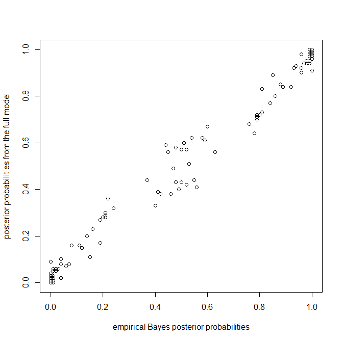
As we might guess - there is more variability when we integrate over the full posterior probability distribution, and this seems to be borne out by our example. We can also compare the posterior probabilities at internal nodes across the two methods. Here's what that looks like:

Again, we're seeing more or less what we'd expect - specifically, more uncertainty in the posterior probabilities from the full model in nodes that have posterior probabilities near zero or one in the empirical Bayesian method.

Cool.

This is just a test version - who knows how many bugs will be found before I'm done; however source code is available here, or (if you'd preferred) it is in a new beta build of phytools (phytools 0.2-53) on my website.

More performance testing on make.simmap

I wanted to repeat & elaborate some performance testing that I conducted earlier in the month. This is partly motivated by the fact that I introduced and then fixed a bug in the function since conducting this test; and partly this is driven by some efforts to figure out why the stand-alone program SIMMAP can give deceptively misleading results when the default priors are used (probably because the default priors should not be used - more on this later).

My simulation test was as follows:

1. I simulated a stochastic phylogeny (using pbtree) and character history for a binary trait with states a and b (using sim.history) conditioned on a fixed, symmetric transition matrix Q. For these analyses, I simulated a tree with 100 taxa of total length 1.0 with backward & forward rate of 1.0.

2. I counted the true number of transitions from a to b & b to a; the true total number of changes; and the true fraction of time spent in state a (for any tree, the time spent in b will just be 1.0 minus this).

3. I generated 200 stochastic character maps using make.simmap. For more information about stochastic mapping or make.simmap search my blog & look at appropriate references.

4. From the stochastic maps, I computed the mean number of transitions of each type; the mean total number of changes; and the mean time spent in state a. I evaluated whether the 95% CI for each of these variables included the true values from 1.

5. I repeated 1. through 4. 200 times.

First, we can ask how often the 95% CI includes the generating values. Ideally, this should be 0.95 of the time:

> colMeans(on95)
   a,b    b,a      N time.a
 0.905  0.895  0.790  0.950

This is not too bad.

Now let's attach some visuals to parameter estimation. Figure 1 shows scatterplots of the relationship between the true and estimated (averaged across 200 stochastic maps) values of each of the four metrics described above:

Figure 1:

Figure 2 is a clearer picture of bias. It gives the distribution of Y - Ŷ, where Ŷ is just the mean from the stochastic maps for a given tree & dataset. The vertical dashed line gives the expectation (zero) if our method is unbiased; whereas the vertical solid line is the mean of our sample.

Figure 2:

That's it. I'm not posting the code - because there's a whole bunch of it; however if you want it, please just let me know.