Method comparison in make.simmap

A couple of days ago I introduced a new version of make.simmap that uses Bayesian MCMC to sample the transition matrix, Q, from its posterior probability distribution rather than fixing it at the MLE (as in previous versions of the function). The idea is that by fixing Q we are ignoring variation in the reconstructed evolutionary process that is due to uncertainty in the transition matrix.

I thought that, as a first pass, it might be neat to compare these two approaches: one in which we fix Q at its most likely value; and the other in which Q is sampled from its posterior probability distribution. My expectation is relatively straightforward - variance on estimated variables should go up (hopefully towards their true variance), and the probability that the generating parameter values should be on their corresponding (1-α)% CIs (which, in general, included less than (1-α)% of generating values in the empirical Bayes method) should go to (1-α).

My analysis was as follows:

1. First, I simulated 200 pure-birth trees containing 100 taxa using the phytools function pbtree. On each tree I simulated the stochastic history of a binary discrete character with two states (a & b) given a symmetric transition matrix with backward & forward rate Q_a,b = Q_b,a = 1.0.

2. For each tree, I computed the number of transitions of each type and of any type; and the fraction of time spent in state a vs. b.

3. Next, for each tree I sampled 200 stochastic character maps conditioning on the MLE transition matrix (Q="empirical").

4. For each set of stochastic maps, I computed the number and type of transitions as well as the time spent in state a and averaged them across maps. I also obtained 95% credible intervals on each variable from the sample of stochastic maps, in which the 95% CI is the interval defined by the 2.5th to 97.5th percentiles of the sample. I calculated the total fraction of datasets in which the true values fell on the 95% CI from stochastic mapping.

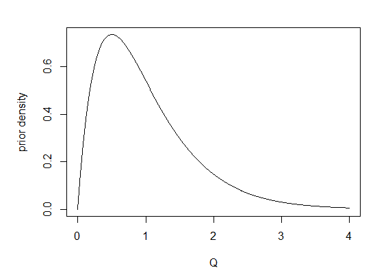
5. Finally, I repeated 1. through 4. but this time stochastic maps were obtained by first sampling 200 values of Q from its Bayesian posterior distribution using MCMC (Q="mcmc"). In this case, I used 1,000 generations of burn-in followed by 20,000 generations of MCMC, sampling every 100 generations. I used a γ prior probability distribution with make.simmap(...,prior(use.empirical=TRUE, beta=2)), which means that the parameters of the prior distribution were β = 2 and α = MLE(Q) × β. The figure below shows the γ prior probability density for α = β = 2.

Here are some of the results. First let's look at the empirical Bayes method in which Q is set to its most likely value:

> ci<-colMeans(on95); ci
   a,b    b,a      N time.a
 0.895  0.925  0.800  0.970
> pbinom(ci*200,200,0.95)
       a,b        b,a          N     time.a
0.00115991 0.07813442 0.00000000 0.93765750

This shows that - although the method is not too bad, the 95% CI coverage is significantly below the nominal level - at least for the number of changes from a to b as well as the total number of changes on the tree.

Now let's see a visual summary of the results across simulations:

Figure 1

Figure 2

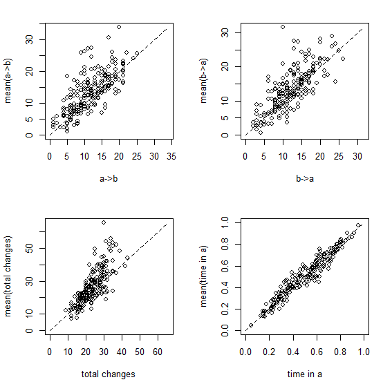
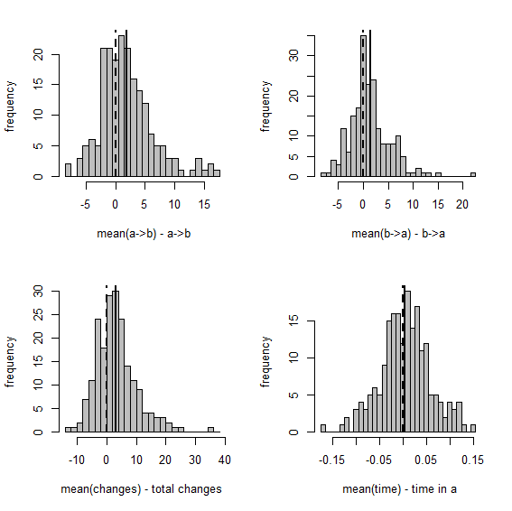
Figure 1 shows a set of scatterplots with the true & estimated values of each of the four variables described earlier. Figure 2 is just a different visualization of the same data - here, though, we have the frequency distribution, from 200 stochastic maps, of the difference between the estimated and generating values.

OK, now let's compare to the full* Bayesian version in which MCMC is used to sample Q from its posterior probability distribution.

(*Note that in a true fully Bayesian method I should not have used my empirical data to parameterize the prior distribution, which I have done here by using prior=list(...,use.empirical=TRUE), but let's ignore that for the time being.)

First, the 95% CI, as before:

> ci<-colMeans(on95); ci
   a,b    b,a      N time.a
 0.970  0.925  0.955  0.940
> pbinom(ci*200,200,0.95)
       a,b        b,a          N     time.a
0.93765750 0.07813442 0.67297554 0.30024430

Neat. This time our (1-α)% CIs include the true values of our 4 variables about (1-α)% of the time; and in no case is this significantly lower than we'd expect by chance.

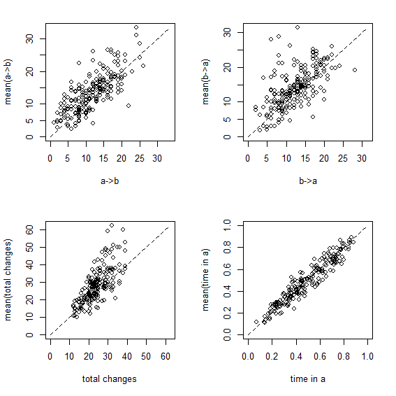
Here are the same two visualizations as for the empirical Bayes method, above:

Figure 3

Figure 4

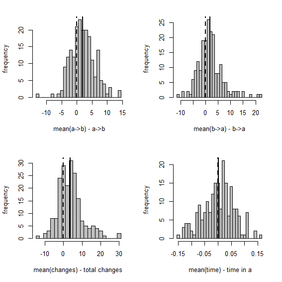
Overall, this shows us that integrating over uncertainty in Q - at least in this simple case - does have the desired effect of expanding our (1-α)% credible interval to include the generating values of our variables in (1-α)% of simulations. Cool.

Unfortunately, make.simmap(...,Q="mcmc") is very slow. I have some ideas about a few simple ways to speed it up and I will work on these things soon.