Fast ML estimation of ancestral states for a continuously valued trait

I just wrote a new function for ancestral character estimation that takes advantage of the fact that the ancestral value for the root node computed during the calculation of independent contrasts is also the MLE of the root. Re-rooting at all internal nodes and the recomputing the PIC root state, cumbersome as it sounds, is actually much faster than finding ancestral states via numerical optimization of the likelihood. The main part of the code for this function is therefore as follows:

M<-btree$Nnode
N<-length(btree$tip)
anc<-vector()
for(i in 1:M+N){
  anc[i-N]<-ace(x,multi2di(root(btree,node=i)), method="pic")$ace[1]
  names(anc)[i-N]<-i
}

Obviously, although this function is designed as a faster version of ace(...,type="continuous",method="ML"), the function actually runs by using many calls to ace(...,method="pic")!!

The object name btree in this code is used to denote binary tree. This highlights the fact that, obviously, contrasts can only be computed for bifurcating trees. We would still like our function to run, though, if the tree contains multifurcating. The remainder of the function code is dedicated to, first, changing a multifurcating tree to a bifurcating one; and then, after computing ancestral states using the code given above, lining up the nodes on the binary tree to the nodes of the original tree containing multifurcations.

The way a did this is a little ad hoc, but it seems to work. I basically went through all the nodes on both the binary and multifurcating tree and, for each node, pulled out a list of all the descendant tips. Then, I used these lists of descendant tips to match nodes between trees.

The code for this function, fastAnc, is here. Let's try it and compare to both ape::ace and phytools::anc.ML.

> library(phytools)
> # first, simulate bifurcating tree & data
> tree<-rtree(200)
> x<-fastBM(tree)
> # now load the source & estimate states with each function
> source("fastAnc.R")
> system.time(res1<-ace(x,tree,method="ML")$ace)
  user  system elapsed
 19.69    0.05   20.38
> system.time(res2<-anc.ML(tree,x,maxit=10000)$ace)
  user  system elapsed
236.67    0.34  255.00
> system.time(res3<-fastAnc(tree,x))
  user  system elapsed
  2.60    0.00    2.98
> # plot to compare
> par(mfrow=c(2,1),mai=c(1.02,0.82,0.1,0.1))
> plot(res1,res3,xlab="ace",ylab="fastAnc")
> plot(res2,res3,xlab="anc.ML",ylab="fastAnc")

Obviously, we get the same estimates from each function - but at much greater computational cost (particularly for anc.ML, which is pretty terrible).

That was for a fully bifurcating tree. We can also do a smaller example to make sure we are back-translating our node IDs correctly. Let's try it:

> tree<-rtree(12)
> # collapse two shortest branches into multifurcations
> tree<-di2multi(tree,tol= sort(tree$edge.length[tree$edge[,2]>length(tree$tip)])[3])
> plot(tree,no.margin=TRUE); nodelabels()

> # simulate data
> x<-fastBM(tree)
> # estimate ancestral states using the three methods
> res1<-ace(x,tree,method="ML")$ace
Error in ace(x, tree, method = "ML") :
 "phy" is not rooted AND fully dichotomous.
> res2<-anc.ML(tree,x)$ace
> res3<-fastAnc(tree,x)
> par(mai=c(1.02,0.82,0.2,0.2))
> plot(res2,res3,xlab="anc.ML",ylab="fastAnc")
> res2
        13          14          15          16          17
0.28663746  0.05138613 -0.25089177  0.50494223  0.13529718
        18          19          20          21
0.03920500  0.49088849  1.24192050  1.63727735
> res3
        13          14          15          16          17
0.28665585  0.05139666 -0.25089395  0.50494620  0.13528936
        18          19          20          21
0.03920408  0.49088277  1.24191236  1.63727663

First off - ace doesn't work at all if the tree is not bifurcating (not sure why this is). anc.ML works fine, but will be very slow for large trees (as we've discovered). fastAnc gives the same estimates and node names - even though it had to first convert to a bifurcating tree, and then back-translate the node numbers. Great!

New version of phytools on CRAN

I just submitted a new version of phytools (version 0.2-0) to CRAN. This is basically the same as the latest "non-CRAN" release (0.1-98) with a couple of minor changes and corrections in the manual pages and to the function fancyTree. However, there have been lots of new additions and changes to phytools since the last CRAN update, version 0.1-9. Here's a (probably non-comprehensive) sample:

1) A new function, threshBayes, to analyze the threshold model from quantitative genetics (described here and here).

2) A new function, bmPlot, for visualizing Brownian motion evolution (here) and evolution under the threshold model (here).

3) A bug fix in the important phytools function nodeHeights (here).

4) An update to the canonical correlation analysis function phyl.cca, as well as some other things (described here).

5) Renaming & movement of the likelihood function for joint Pagel's λ for multiple characters to the NAMESPACE (described, along with instructions for using this function - likMlambda - to perform joint estimation of Pagel's λ, here).

6) Minor update to phylogenetic principal components function, phyl.pca (here).

7) New version of fitDiversityModel with much improved likelihood estimation (described here).

8) New tree plotting method in the function fancyTree (here) along with various improvements thereof (here).

9) A number of changes to documentation and some minor fixes and updates to internal phytools functions.

The source build of phytools 0.2-0 is already available from CRAN (although will not yet have percolated through all mirrors), and from my phytools page. Obviously, it may take a few days for Mac OS and Windows binaries to be available.

read.simmap: computation time rises more than linearly with the number of trees

Sam Price reports that computation time for phytools function read.simmap(...,version=1.5) rises more than linearly with the number of trees in the input file. That means that it takes (substantially) more than twice as long to read in a data file containing 200 trees than it does to read in a data file containing 100 trees. (Or, equivalently, it would be faster to split your trees into two files and then read them in separately.)

Well, it turns out that Sam is right, of course - but I haven't yet figured out why. If I have time, I will try and figure this out tomorrow. Here is the result of reading in tree files with various numbers of trees using read.simmap and timing the result using system.time (if it seems slow it is because I am running it on my VAIO ultrabook):

Modification to fancyTree(...,type="droptip") so that it works on non-ultrametric trees

In response to a phytools user comment I gave a trick (here) for plotting the leaves and edges to be dropped in a different color & style from the rest of the tree. I then incorporated this trick into the phytools function fancyTree (described here). What I failed to point out was that this trick will not work on non-ultrametric trees. (To be honest, it didn't even really occur to me to point this out, so jaded am I from working with simulated data and trees.) Well, I have fixed this now, so that fancyTree(...,type="droptip") no longer uses the trick I described here, although it does still, generally speaking, use the method of fancyTree(...,type="extinction").

Users can check out the updated code on my R phylogenetics page here; or just download the latest (non-CRAN) version of phytools (v0.1-98: here), and install from source.

Let's check out how it works:

> # install new version of phytools, if necessary
> install.packages("phytools_0.1-98.tar.gz",type="source", repos=NULL)
> # simulate non-ultrametric tree & drop tips
> set.seed(10)
> tree<-rtree(n=20)
> pruned<-fancyTree(tree,"drop",tip=sample(tree$tip)[1:5])

Well, that works great. The only thing I'm not satisfied with is that if pruning changes the total length of the tree, then the second panel will be automatically rescaled so that corresponding nodes in the two plotted trees no long have corresponding horizontal positions. For example:

> set.seed(100)
> tree<-rtree(n=20)
> tips<-c("t6","t8","t14","t12","t4","t20")
> pruned<-fancyTree(tree,"drop",tip=tips)

Still working on this. . . .

Matching partial strings

To allow users to specify plot type (argument type) in the phytools function fancyTree without having to write the string for the desired type out in full, I yesterday wrote a custom function to match partial strings - the internal phytools function matchType. This is what it looked like:

matchType<-function(type,types){
 for(i in 1:length(types))
  if(all(strsplit(type,split="")[[1]]==strsplit(types[i], split="")[[1]][1:length(strsplit(type,split="")[[1]])]))
   type=types[i]
 return(type)
}

The very long if statement basically asks if (when type is split into a character vector with strsplit) all it elements (up to its total length) match all the elements of the current type under evaluation. So, for instance, we can do the following:

> type="extinct"
> matchType(type,c("extinction","traitgram3d","droptip"))
[1] "extinction"
> type="drop"
> matchType(type,c("extinction","traitgram3d","droptip"))
[1] "droptip"

or any number of a virtually infinite number of variations thereof.

It did strike me, though, that there might be a pre-existing R function to do this - and sure enough, there is: pmatch in the base package. It is slightly different from matchType in that it returns the index of the (partially) matching strings, but it is otherwise pretty much identical. To use it as a substitute for matchType, we would just have to do the following:

> types=c("extinction","traitgram3d","droptip")
> type="extinct"
> types[pmatch(type,types)]
[1] "extinction"
> type="drop"
> types[pmatch(type,types)]
[1] "droptip"

Sigh - oh well!

New option in fancyTree to plot tree pruning

I just added the code snippet from yesterday as a additional option to the phytools function fancyTree (previously described here, here, and here). A link to the source code for the new function is here.

Now, fancyTree, which is the function into which I'm dropping my efforts to make it easier for R phylogenetics users to plot various types of specialized phylogenies, has three different options (specified by the option type):

1) type="extinction": this method, described here, plots branches leading only to extinct taxa, and branches before the MRCA of all extant species in the tree, using red dashed lines (whereas all the other branches are plotted in black). For example:

> set.seed(10)
> tree<-rlineage(1,0.5,4)
> fancyTree(tree,type="extinction")

2) type="traitgram3d": this method, described here, uses phytools::phylomorphospace3d to plot a three dimensional 'traitgram'. For instance:

> tree<-pbtree(n=50,scale=10)
> Y<-sim.corrs(tree,vcv=matrix(c(1,0.75,0.75,1),2,2))
> fancyTree(tree,type="traitgram3d",X=Y, control=list(spin=FALSE))

3) Finally, the newest addition, type="droptip": this method takes the tree and set of tips to drop, and then plots the branches to be pruned in a separate color. Finally, it returns the pruned tree. For instance:

> tree<-pbtree(n=30)
> tips<-sample(tree$tip.label)[1:10]
> pruned<-fancyTree(tree,type="droptip",tip=tips)

I have added this new version of fancyTree to phytools. The new package version (v0.1-97), which can be downloaded and installed from source, is here.

> install.packages("phytools_0.1-97.tar.gz",type="source", repos=NULL)
Installing package(s) into ...
...
* DONE (phytools)
> library(phytools)

Plotting with the leaves and edges to be dropped highlighted

An anonymous reader commented the following:

I am wondering, is it possible to give different colours to the taxa after pruning by using the drop.tip. I just want to show the locations of the used species in the whole tree. All the taxa in tree retains but with different colours? (e.g. used species blue or red and pruned ones grey)

Ok, I'm going to interpret this as meaning - can we paint the leaves and edges that we're going to drop from the tree a different color, plot these, then drop them? (Once we've dropped these tips and edges from the tree, they are really gone - so we definitely can't plot them any more at that point.)

The answer is, of course, yes - and I'm going to give a quick trick for doing this using functions from the packages phytools (my package, of course) and ape.

Here I go. For the purposes of illustration, I will use a simulated, 30-taxon ultrametric tree; and a random set of ten tips.

> # first simulate a tree > tree<-pbtree(n=30) > # choose a random set of tips to prune > tips<-sample(tree$tip.label)[1:10] > tips [1] "t20" "t8" "t17" "t9" "t15" "t2" "t13" "t14" "t16" [10] "t11" > # find the node numbers for those tips > nodes<-sapply(tips,function(x) which(x==tree$tip.label)) > # and the rows in our edge matrix for all terminal branches > # to be dropped > edges<-sapply(nodes,function(x) which(x==tree$edge[,2])) > # now let's shorten them by an imperceptible amount > tree$edge.length[edges]<-tree$edge.length[edges]- 0.0001*max(nodeHeights(tree)) > par(mfrow=c(2,1)) > # plot the tree using fancyTree in phytools > fancyTree(tree) > # drop tips and plot the pruned tree > tree<-drop.tip(tree,tips) > fancyTree(tree)

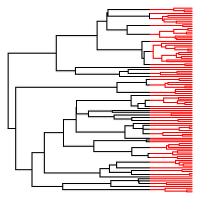
Pretty cool! The way this works is by identifying and then imperceptibly shortening the terminal edges leading to species that we plan to drop from the tree. We can then use the phytools function fancyTree(...,type="extinction") to automatically detect these species (as well as any internal branches leading to these species) as "extinct." It then plots all these edges with red dashed lines, instead of the standard black. (We could modify these color scheme - but as of now we'd have to change the function code).

That's it! Thanks for the suggestion.

How to read in a vector stored as a R expression in a text file (and other things)

A Facebook friend asked:

R question: I have a file that contains a list of entries of the format "c(2.34306542445513, 1.07370083005978e-06)". How can I coax R to read such entries literally? In other words, I want to make an object from the entries. pars <- c(2.34306542445513, 1.07370083005978e-06)

My first response was to do this the hard way. Let's say we have a text file with one or multiple rows as described:

c(2.34306542445513, 1.07370083005978e-06) c(0.71697056549601, 0.03731942130253) c(1.29112553643060, 1.41375523433091) c(0.1173946523107, 0.14024055395275)

Before realizing that there is a much easier way, I pointed out that we can do what's been proposed using readLines, strsplit, paste, and as.numeric. I include this primarily to emphasize how easy it :

> y<-readLines("datafile.txt",4) > x<-strsplit(y,"") > x<-lapply(x,function(x) paste(x[3:(length(x)-1)], collapse="")) > x<-lapply(x,function(x) strsplit(x,", ")[[1]]) > X<-sapply(x,as.numeric) > X [,1] [,2] [,3] [,4] [1,] 2.343065e+00 0.71697057 1.291126 0.1173947 [2,] 1.073701e-06 0.03731942 1.413755 0.1402406

Anyway, shortly after posting this I realized that this could be done much more easily using the functions eval and parse:

> y<-readLines("datafile.txt",4) > X<-apply(as.matrix(y),1,function(x) eval(parse(text=x))) > X [,1] [,2] [,3] [,4] [1,] 2.343065e+00 0.71697057 1.291126 0.1173947 [2,] 1.073701e-06 0.03731942 1.413755 0.1402406

That's it!

P.S. please let me know if you prefer this new "text box" format for R code and session results, or my previous method of font only based demarcation (e.g., shown here, and in almost any other post on this blog).

New version of fitDiversityModel with vastly improved ML optimization & correct covariance matrix for parameter estimates

I just posted a new version of the function fitDiversityModel. This function does the main part of the analysis of Mahler et al. (2010), but with some modifications. Most importantly, Mahler et al. use REML; whereas this function does ML. (In addition, in the paper there were some issues in the way in which we computed ecological opportunity at internal nodes. This has been fixed in the form of the phytools function estDiversity - although this is not directly relevant to fitDiversityModel, which can theoretically fit our opportunity model with ecological lineage densities from any source.)

This function is designed to fit a model of character evolution for a single trait in which the rate of Brownian evolution changes as a function of the lineage density** at internal nodes of the tree (**or any other feature that we can track for nodes on the tree). Consequently, the model has two main parameters of interest: σ₀², the starting rate of evolution; and what we called "ψ", the rate of gain or loss in the BM rate per unit of change in ecological opportunity. If ψ < 0, this would indicate that the rate of evolution declined as lineages were added within an ecological community.

In using the previous version of fitDiversityModel for some new analyses, Luke Mahler discovered that fitDiversityModel was sensitive to the scaling of the tree. Theoretically, this should not be the case. For instance, if we scale the tree by a factor of 2, then we should expect σ₀² and ψ to half. In fact, we can see this to be true (the data here are PC1 from the Mahler et al. paper, I believe).

> library(phytools)
> library(geiger)
> res1<-fitDiversityModel(rescaleTree(tree,1),x,d=density)
> res1
$logL
[1] -7.782838
$sig0
[1] 0.237636
$psi
[1] -0.003973024
$vcv
            sig0          psi
sig0  0.001622423 -0.002161093
psi  -0.002161093  0.009471374
$convergence
[1] TRUE
> res2<-fitDiversityModel(rescaleTree(tree,2),x,d=density)
> res2
$logL
[1] -7.782838
$sig0
[1] 0.118824
$psi
[1] -0.001986653
$vcv
            sig0          psi
sig0  0.000405508 -0.001080177
psi  -0.001080177  0.009469173
$convergence
[1] TRUE

[A quick sidenote on why we expect our likelihoods to be constant for rescaled trees - but not for rescaled data, for instance. The expected multivariate distribution of our tip data on the tree is always a function of the branch lengths of the tree × parameters in our evolutionary model. Thus, by scaling branch lengths up & evolutionary parameters down (or vice versa) we always end up the same multivariate probability density.]

OK, so far so good. But what about a more dramatic rescaling? If we scaled our tree by 100 instead of 2, we should just expect our parameter estimates to change by 1/100 instead of 1/2, right? Unfortunately, Luke discovered that as we rescale the branch lengths up it becomes increasingly difficult for optim, the base package multivariate optimizer, to converge on the correct solution. For instance:

> res100<-fitDiversityModel(rescaleTree(tree,100),x,d=density)
> res100
$logL
[1] -13.69297
$sig0
[1] 0.001646267
$psi
[1] 0
$vcv
             sig0          psi
sig0 -2.298157e-09 5.825806e-05
psi   5.825806e-05 3.639800e-01
$convergence
[1] FALSE

Initially, I tried to solve this by tweaking the control of optim, but then I realized that we had analytic solutions for σ₀² and (the other parameter in the model, the ancestral state at the root node) a conditioned on ψ - so the problem could pretty easily be reformulated as a univariate, rather than multivariate, optimization problem. This could pretty much immediately take care of optimization issues, because the univariate optimizer (optimize) is much more reliable and quicker than optim.

So, I have updated fitDiversityModel to perform univariate optimization of ψ & use conditional MLEs for σ₀² and a, and it works great! The code for this function is here, but I would generally advise installing the new version of phytools from source (here). This is because phytools imports a function, hessian, from the 'numDeriv' package, via the NAMESPACE, and this will generally not be available to fitDiversityModel unless it is loaded as part of the package.

[Note that although you can detach phytools to install and load the new version, I find that it is generally better to start a new R session here.]

> install.packages("phytools_0.1-96.tar.gz",type="source", repos=NULL)
> library(phytools)
> library(geiger)
> res1<-fitDiversityModel(rescaleTree(tree,1),x,d=density)
> res1
$logL
[1] -7.782838
$sig0
[1] 0.2376324
$psi
[1] -0.003972944
$vcv
             sig0           psi
sig0  0.0016200023 -3.757170e-05
psi  -0.0000375717  1.027241e-06
> res100<-fitDiversityModel(rescaleTree(tree,100),x,d=density)
> res100
$logL
[1] -7.782838
$sig0
[1] 0.002376324
$psi
[1] -3.972944e-05
$vcv
             sig0           psi
sig0  1.620002e-07 -3.757170e-09
psi  -3.757170e-09  1.027241e-10

Now the function is behaving a lot better - users should also notice that it is markedly faster (about 3 × faster if showTree is turned off).

A second thing the user might notice, though, is that the covariance matrix of the parameter estimates from the Hessian has changed as well. What happened? Well, it turns out this was a real bug with fitDiversityModel in its prior iterations. [I'm not characterizing the other problem as a real bug because fitDiversityModel warned us that it had not converged!] The problem was that internally fitDiversityModel was rescaling ψ for better optimization; and although ψ was backtransformed to its original scale for output, the variance of ψ was not! This is a pretty significant oversight, but it should've only affected people using $vcv to compute, say, a 95% confidence interval on model parameters (likelihood-ratio tests and AIC would not have been affected).

I also made one final change to the function - also affecting how ψ is rescaled internally. Basically, this will only affect your results if the range of values in d was very small, but the effect of d was large. We discovered this problem when we used "time since the root" as our d vector. In this case if the total tree length was short (e.g., 1.0 instead of, say, 100) parameter estimates could be off.

Using ltt on a set of trees, plus a cool animation

A phytools user just commented that it would be cool to be able to automate the calculation of Pybus & Harvey's γ statistic for a set of phylogenies (say, a posterior sample of trees from a Bayesian analysis). This is actually already pretty easy - just do the following (trees is a set of trees stored in an object of class "multiPhylo"):

g<-sapply(trees,function(x) ltt(x)$gamma)

For example, let's try it on a set of pure-birth phylogenies simulated using phytools::pbtree:

> library(phytools)
> trees<-pbtree(n=100,nsim=1000,scale=1)
> g<-sapply(trees,function(x) ltt(x)$gamma)
> # gamma should be standard normal for Yule trees
> mean(g)
[1] -0.04430857
> var(g)
[1] 0.9603543
> hist(g,main="Pybus' gamma on pure-birth trees")

Cool.

Running ltt on a set of trees also incidentally creates a neat animation. Here's what it looked like for my 1000 simulated trees (more or less - I added the counter & diagonal reference line for effect):



That's it!

Including the phenotypes of fossil taxa in the estimation of phylogenetic signal

A phytools user asks:

Does the phylosig function [Ed. for the estimation of phylogenetic signal] work for non-ultrametric trees? Can I include fossils in my phylogeny?

The answer to both these questions is "yes"? With regard to the former inquiry: I can see two main reasons for using a non-ultrametric tree in the computation of phylogenetic signal. The first is that we have some a priori reason to believe that the rate of character evolution differs strongly on different branches of the tree and we want to condition on this rate heterogeneity. The second is that we have extinct taxa (lineages terminating before the present) included in our phylogeny. In both cases we can compute phylogenetic signal for our characters of interest in the usual way.

The second question pertains to including fossil data in the phylogeny. If the user is referring to the practice of including extinct taxa (fossil species) as lineages terminating before the present, then I have already answered the question. However, if what he or she wants to do is attach a datum (or multiple data) to a specific node or to a point along an internal edge, then this is a different matter. Again, it is possible, but a tiny bit more complicated.

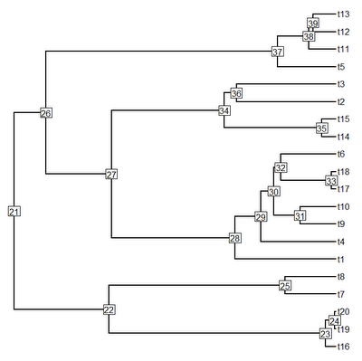
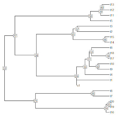
The easiest way to do this is by attaching an extra branch of zero length to our tree. If the fossil placement is at an internal node, then we attach the branch to the node as follows (note that I'm going to do this by simulation using phytools::pbtree, but to repeat this, the user has to update phytools to the latest non-CRAN version, v0.1-95, here - also see note at the end of this post):

> library(phytools)
> # first, let's say we have a phylogeny with 20 tips
> tree<-pbtree(n=20)
> # plot the tree with node labels
> plotTree(tree,node.numbers=T,pts=F)

> # ok, now let's assume that our fossil data can be
> # confidently placed at, say, node 28
> # first create a new tip
> tip<-list(edge=matrix(c(2L,1L),1,2),tip.label="x1", edge.length=0,Nnode=1L)
> class(tip)<-"phylo"
> # then attach it
> xtree<-bind.tree(tree,tip,where=28)
> x11(); plotTree(xtree,pts=F,node.numbers=T)

[Note here that all the node numbers have increased by one. This happens even though we have not added any internal nodes to the tree because we have technically added a new tip, and the counting scheme for node numbers begins with number N+1 for N tips in our phylogeny.]

We can repeat this procedure as many times as we want - adding additional fossil phenotypes to the tree.

Normally, then, we would have our data vector containing both the values for all the tip nodes, and the values for ancestral nodes from fossils - the latter named by the convention we have adopted to add new tips to the tree (here, "x1"). Since this is a simulated example, we can just generate some data:

> x<-fastBM(xtree)
> x
        t16         t19   ...          x1
-3.38357132 -3.04220865   ...  0.17339482

So, you can see that the data for tip species and internal nodes are just treated in exactly the same way in the input data vector. We can then compute phylogenetic signal in the normal way:

> phylosig(xtree,x,method="K")
[1] 1.294228
> phylosig(xtree,x,method="lambda")
$lambda
[1] 0.9967708
$logL
[1] -21.76246

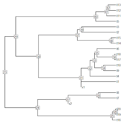
We can do basically the same thing for fossils that we want to place along an edge of the tree, instead of directly at a node. In this case, we would do the following:

> # using our tree from before, say we have a fossil that we
> # want to add halfway between (new) nodes 23 & 26
> tip<-list(edge=matrix(c(2L,1L),1,2),tip.label="x2", edge.length=0,Nnode=1L)
> class(tip)<-"phylo"
> # then attach it
> xtree<-bind.tree(xtree,tip,where=26, position=0.5*xtree$edge.length[which(xtree$edge[,2]==26)])
> plotTree(xtree,pts=F,node.numbers=T)

Then we just proceed as before.

**An important addendum is that the simulation using pbtree for phylogeny simulation does not work with the current CRAN version of phytools, and thus to run the simulation exactly as detailed above, one needs to update to the latest non-CRAN phytools version. This is because of although pbtree simulates trees that are (so far as I can tell) compliant with the ape standard, ape::bind.tree nonetheless finds some problem in how edges are numbered and ordered. This will not result in an error - rather a misplacement of the attached tip in the tree. I have built a temporary fix for this problem into the newest version of pbtree, and I may describe that fix in a separate post.

Tanja Stadler "phyloseminar" on estimating speciation & extinction rates on trees

Tanja Stadler, from ETH Zurich, is giving an online web seminar today at phyloseminar.org. Her talk will be about estimating speciation & extinction rates from phylogenies and might be quite interesting to check out. If you haven't watched a "phyloseminar" live before, phyloseminar.org uses EVO - kind of like a fancy, multiuser Skype. The interface is very cool - but you should allow a little extra time before the seminar (scheduled for 1PM eastern) to make sure you get online with no difficulty. If you miss the seminar, you can always watch the recorded version later.

Fitting a shift in the evolutionary rate at a fixed point above the root: a primer

An R-sig-phylo list serve subscriber asked the following:

I was wondering if there is a method to test for varying rates over time.... I was thinking... in terms of testing if there is a different rate for the entire tree after a specified point in time. For instance, if a snail predator colonizes an island 3.4 Mya, is there evidence for an increased rate of evolution in the prey after that point in time?

Matt Pennell, a Ph.D student in the Harmon lab, responded that this could easily be done using the functions of phytools. He's right, and here's a quick primer (surprisingly pronounced "primmer", for some reason, in American English).

> library(phytools)
> # now let's simulate a stochastic tree
> tree<-pbtree(n=100,scale=15)
> # let's map two states on the tree
> # one for the time before 3.4mybp
> tree<-make.era.map(tree,c(0,max(nodeHeights(tree))-3.4))
> plotSimmap(tree,pts=F,lwd=3,ftype="off") # visualize

> # now let's simulate some data (since we don't have any)
> x<-sim.rates(tree,c(1,10))
names absent from sig2: assuming same order as $mapped.edge
> # finally, let's fit our two rate model
> fit<-brownie.lite(tree,x)
> fit
$sig2.single
[1] 8.750253
...
$logL1
[1] -316.6358
...
$sig2.multiple
        1          2
0.6825954 11.3658746
...
$logL.multiple
[1] -310.6544
...
$P.chisq
[1] 0.0005427315
...

That's it.

Update to phyl.pca so that "mode" (correlation vs. covariance) can be specified flexibly

A user recently complained the following about phytools function phyl.pca for phylogenetic principal components:

One little suggestion for protecting users from themselves might to throw up an error if the user misspells the mode parameters [Ed. note: which specifies whether to use the covariance or correlation matrix during analysis]. Currently, if you type:
   mode="cor"
It will work, and just run on the default covariance matrix. But "cor" is a misspelling of "corr", which will yield the desired analysis. It might be a common error, since cov and cor are both three letters. I just did this, but noticed the output was identical.

Good suggestion. I have now added a few lines of code to phyl.pca to fix this problem. Basically, the function now accepts any unambiguous shorting of covariance and correlation instead of just the three and four letter strings "cov" and "corr" respectively. In addition, if the match is imperfect, the function will return a message.

The updated function code is here; it is also in the latest non-CRAN version of phytools (v0.1-94, here) and will be in the next CRAN phytools release.

The way I achieved this is really simple. Basically, I used the base function strsplit to split the input mode into characters; then I matched the specified mode characters to strsplit("correlation",split="") or strsplit("covariance",split=""). Finally, if the match was imperfect (for instance, mode="corelation"), the function defaults to using the covariance matrix, but also spits an error.

Here's a demo:

> # first install new phytools
> install.packages("phytools_0.1-94.tar.gz",type="source", repos=NULL)
Installing package(s) into ‘C:/Users/liam.revell/Documents/R/win-library/2.14’ (as ‘lib’ is unspecified)
* installing *source* package 'phytools' ...
> # load phytools
> library(phytools)
> # for demo, simulate tree & data
> tree<-pbtree(n=40,scale=100)
> L<-matrix(rnorm(n=16),4,4); L[upper.tri(L,diag=F)]<-0
> V<-L%*%t(L) # covariance matrix for simulation
> X<-sim.corrs(tree,V)
> X
          [,1]        [,2]         [,3]       [,4]
t1   10.0145660  25.5508968  27.14419359 -16.670596
t2   -0.9504677  -1.1381218  23.31553654 -16.947086
t3         ....
> pca<-phyl.pca(tree,X,mode="covar")
> pca<-phyl.pca(tree,X,mode="co")
mode = 'co' not a valid option; setting mode = 'cov'
> pcaCorr<-phyl.pca(tree,X,mode="corelation")
mode = 'corelation' not a valid option; setting mode = 'cov'
> pcaCorr<-phyl.pca(tree,X,mode="correlation")
> pca
$Eval
        PC1      PC2      PC3          PC4
PC1 5.612471 0.000000 0.000000 0.000000e+00
PC2     ....
$Evec
           PC1        PC2       PC3         PC4
[1,] -0.2026469  0.2849556 0.1557432  0.92383906
[2,] -0.5305595  0.6617452 0.3666632 -0.38230631
[3,] -0.4710700 -0.6810988 0.5603986  0.01227893
[4,]  0.6749325  0.1303764 0.7261237 -0.01457757
$S           PC1        PC2         PC3          PC4
t1  -24.731226  -0.357717  13.5570211  0.038474777
t2        ....

> pcaCorr
$Eval
        PC1      PC2       PC3          PC4
PC1 2.363718 0.000000 0.0000000 0.000000e+00
PC2     ....
$Evec
           PC1        PC2       PC3         PC4
[1,]  0.5945738  0.3526378 0.1810304  0.69954028
[2,]  0.6090435  0.3035288 0.1661745 -0.71366821
[3,]  0.2450079 -0.7643208 0.5960410  0.02280308
[4,] -0.4642405  0.4464644 0.7644274 -0.02830375
$S
          PC1         PC2         PC3          PC4
t1   16.705476  -3.6663012   7.3051355  0.040978169
t2        ....

That's it. Thanks to the phytools user for his comment. Keep them coming!

Addendum to estimating ancestral states under an OU model

In a follow up to the R-sig-phylo thread that initiated yesterday's thread, an R phylogenetics user report that the method fails for high values of α with the error report that the among-species VCV matrix was singularity or nearly so. My guess is that this is due to the optimizer trying values of σ² which cause the matrix to be numerically indistinguishable from singular. Singular matrices, of course, cannot be inverted, which will cause the likelihood calculations to fail.

Luckily, there is an alternative approach, as I report in my response to this message. Specifically, we can take advantage of the fact that the state for the root node of the tree computed during Felsenstein's independent contrasts algorithm also corresponds to the MLE for that node. We can thus go through all the nodes of the tree, each time re-rooting the tree at that node and computing its MLE ancestral character estimate by obtaining the PIC state for this new "root."

Here's how we might do this for phylogeny tree and data vector x:

> # first estimate alpha under the OU model
> fit<-fitContinuous(tree,x,model="OU")$Trait1
Fitting OU model:
> ou<-vector(); N<-length(tree$tip); M<-tree$Nnode
> # transform the tree by alpha
> outree<-ouTree(tree,fit$alpha)
> # compute the PIC "root" state for each internal node
> for(i in 1:M+N){
   ou[i-N]<-ace(x,multi2di(root(outree,node=i)),
      method="pic")$ace[1]
   names(ou)[i-N]<-i
 }

Simple as that. This will give the same estimates as ace(...,method="ML") (or, for that matter, phytools::anc.ML) for conditions in which the likelihood can be maximized by R.

Note that for some reason that is not completely clear to me root(...,resolve.root=TRUE) and multi2di(root(...)) don't yield the same tree & branch lengths - the latter being what we need in this case.

Estimating ancestral states under a single-optimum OU model

In a recent R-SIG-phylo thread, a R phylogenetics user inquired about how to obtain ancestral state estimates for internal nodes based on an Ornstein-Uhlenbeck model for trait evolution on the tree. They pointed out that, in principle, it should be possible to do this using ace(...,method="GLS",corStruct=corMartins(...)); unfortunately this was not producing sensible ancestral character estimates (and I wasn't able to get it to work at all, for some unknown reason).

Without judging the wisdom of this general endeavor (which I'll discuss a little at the end of this post), I provided a relatively straightforward way to do this using ace(...,method="ML") combined with geiger::fitContinuous and geiger::ouTree. Basically, we first fit our OU model using fitContinuous(...,model="OU"), then we transform the branch lengths of our tree using ouTree(...), finally we estimate ancestral states using ace in the 'ape' package or phytools::anc.ML.

Just to demo this, I'll simulate and estimate below:

> # load the required libraries
> library(phytools) # also loads ape
> library(geiger)
> # set the conditions for simulation
> N<-50; alpha<-1
> # simulate our tree
> tree<-pbtree(n=N,scale=10)
> # simulate data, including internal nodes
> # under a single-optimum OU model
> x<-fastBM(ouTree(tree,alpha),internal=TRUE)
> # fit using geiger::fitContinuous
> fit<-fitContinuous(tree,x[1:N],model="OU")$Trait1
Fitting  OU model:
> fit
$lnl
[1] -46.27052
$beta
[1] 0.7832121
$alpha
[1] 0.9540822
$convergence
...

> # estimate ancestral states
> ou<-ace(x[1:N],ouTree(tree,fit$alpha))
...
> ou$ace
         51           52           53           54
0.012733299  0.012733173  0.012733128          ...
> # or ou<-anc.ML(ouTree(tree,fit$alpha),x[1:N])
> # check how we did
> cor(x[names(ou$ace)],ou$ace)
[1] 0.8046332
> plot(x[names(ou$ace)],ou$ace,xlab="true states",ylab="estimated states")

Because these are simulated data, we can also check to see how well we did - and it turns out that we did a little bit better than we might have if we'd assumed BM as the generating model:

> bm<-ace(x[1:length(tree$tip)],tree)
> cor(x[names(bm$ace)],bm$ace)
[1] 0.6990525
> plot(x[names(bm$ace)],bm$ace,xlab="true states",ylab="estimated states")

Of course, the whole exercise might be a somewhat questionable endeavor. This is because in a single optimum OU model we can't separately estimate the ancestral state at the root node and the position of the phenotypic optimum. That means that we have to be pretty comfortable with assuming that the ancestor of our group was at the trait optimum, which may or may not have been the case depending on our data and tree.

That's it.

New 'Evolution' paper out - and we made the cover!

My new paper with Graham Reynolds describing a new Bayesian method for fitting evolutionary models to comparative data with intraspecific variation (entitled, creatively, "A new Bayesian method for fitting evolutionary models to comparative data with intraspecific variation") has now come out in the journal 'Evolution' (link to September table of contents, here). Not only that, but we made the cover!

The method of this article is implemented in the phytools function fitBayes and described in a prior post to this blog. Check it out!

Joint estimation of Pagel's λ for multiple characters

In a previous post, I described adding a previously internal function for computing the likelihood of a single value of λ for multiple traits to the NAMESPACE of phytools. This function (likMlambda) can now be used in a very simple way to find the ML joint λ estimate for multiple characters. This is described (if I remember correctly) in Freckleton et al. (2002) and implemented internally in the phytools functions phyl.cca & phyl.pca, but not in any stand alone functions. Here is the function:

joint.lambda<-function(tree,X){
  result<-optimize(f=likMlambda,X=X,C=vcv(tree),interval=c(0,1),     maximum=TRUE)
  return(list(lambda=result$maximum,logL=result$objective[1]))
}

Let's try it out:

> tree<-pbtree(n=100)
> X<-fastBM(lambdaTree(tree,0.7),nsim=10)
> joint.lambda(tree,X)
$lambda
[1] 0.6722762
$logL
[1] -1816.575

Pretty cool.

New version of phyl.cca and some other updates

First off, I've had a small number of user comments about phyl.cca (my function for phylogenetic canonical correlation analysis; see Revell & Harrison 2008). One is that the rows of the input data matrices have to be in the same order as the tip labels in the tree. I can find no reason why this should be the case (and was not able to replicate the problem with simulating and randomly permuted data), but I have made some changes to the function in the way that the rows of X & Y are sorted, so hopefully this eliminates the problem.

In troubleshooting this bug, however, I also discovered a more serious issue. phyl.cca can perform joint estimation of λ prior to CCA. The problem is that in previous version of the function I computed log(det(V)) instead of determinant(V,logarithm=TRUE). Why is this significant? Well, for trees of even a modest size (and depending on the scale of the tree), det(vcv.phylo(tree)) goes to 0 or Inf pretty easily. This makes log(det(vcv.phylo(tree))) -Inf or Inf, respectively. Since this can sometimes be true over the entire range of λ, this means we will have no power to estimate λ. I've realized that this can be a problem in likelihood calculation for quite some time, so all my other functions computing the log-likelihood use determinant(...,logarithm=TRUE), but until recently I didn't realize this might not have been fixed in phyl.cca. (It is also a problem in phyl.pca since both functions use the same function for computing the likleihood.)

A quick note to users - R automatically spits errors for these calculations at the limit of numerical precision, so you would probably have to have ignored these for this to have been a problem in your analyses. This bug was still somewhat difficult to detect - particularly for phyl.cca, as this function did not previously return the log-likelihood of the fitted λ model.

I also moved the code for the likelihood function for joint λ estimation out of the source files phyl.cca.R & phyl.pca.R, and into a common source file utilities.R. All are available on my phytools page, but a better move for updating the functions would be to install the latest non-static (i.e., non-CRAN) version of phytools, v0.1-93 (here). Remember, to install from source, just download the package zipped tarball, and then type:

> install.packages("phytools_0.1-93.tar.gz", type="source", repos=NULL)

All the affected functions should work just as they did before - if users find that this is not the case, please do report it! The only difference should be that (1) the bug is fixed; and (2) that phyl.cca now reports the log-likelihood of the fitted joint λ model (as mentioned above). To give you a sense of what this looks like, I'll demo the function with some simulated (in this case, uncorrelated) data.

> require(phytools)
> require(geiger)
> tree<-pbtree(n=100)
> X<-fastBM(lambdaTree(tree,0.7),nsim=5)
> Y<-fastBM(lambdaTree(tree,0.7),nsim=4)
> cca<-phyl.cca(tree,X,Y,fixed=FALSE)
> cca
$cor
[1] 0.31327528 0.24224365 0.19474713 0.05333107
$xcoef
           CA1        CA2        CA3         CA4
[1,] -0.5431358  0.2006402 -0.2864722 -0.66959452
[2,] -0.5769728 -0.7635696 -0.4518404  0.39029667
...
$lambda
      lambda          logL
   0.6496061 -1502.6777738
$chisq
[1] 19.296734  9.586766  3.902187  0.267736
$p
[1] 0.5026200 0.6521626 0.6899113 0.8747055

One thing worthy of noting is that (as with many comparative tests) we tend to get very high type I error rates both if phylogenetic signal is simulated and ignored; or if phylogenetic simulation is not simulated, but assumed. For example:

> # first, simulate with phylogenetic signal
> # but conduct standard (i.e., non-phylogenetic) CCA
> X<-fastBM(tree,nsim=5)
> Y<-fastBM(tree,nsim=4)
> cca<-phyl.cca(tree,X,Y,lambda=0,fixed=TRUE)
> cca
$cor
[1] 0.4475067 0.4013825 0.2543455 0.1886160
...
$lambda
 lambda     logL
   0.00 -1582.95
$chisq
[1] 47.211293 26.204985  9.691704  3.405079
$p
[1] 0.0005482501 0.0100392599 0.1382499000 0.1822202083

> # now incorporate phylogeny
> cca<-phyl.cca(tree,X,Y)
> cca
$cor
[1] 0.3510597 0.2884059 0.1348753 0.1122388
...
$lambda
  lambda      logL
   1.000 -1131.117
$chisq
[1] 23.443939 11.080562  2.917425  1.191692
$p
[1] 0.2675254 0.5220274 0.8191373 0.5510960

> # now do the converse - simulating without signal
> X<-fastBM(lambdaTree(tree,0),nsim=5)
> Y<-fastBM(lambdaTree(tree,0),nsim=4)
> cca<-phyl.cca(tree,X,Y)
> cca
$cor
[1] 0.78268746 0.50448553 0.33628950 0.09279904
...
$lambda
  lambda      logL
   1.000 -2276.737
$chisq
[1] 128.8425842  39.7027005  12.0941745   0.8130019
$p
[1] 6.424246e-18 8.055169e-05 5.990056e-02 6.659765e-01

> # now estimate using standard (non-phylogenetic) CCA
> cca<-phyl.cca(tree,X,Y,lambda=0,fixed=TRUE)
> cca
$cor
[1] 0.38150517 0.23933981 0.11302862 0.04147243
...
$lambda
  lambda      logL
   0.000 -1765.266
$chisq
[1] 21.7010083  6.9154811  1.3704468  0.1618157
$p
[1] 0.3569526 0.8631480 0.9676315 0.9222787

The final thing I did was add the likelihood function for joint λ to the NAMESPACE of phytools. This enables the phytools user to write an incredibly simple function for joint λ estimation. I will detail this in a separate post (to improve search).

Phylogenetic signal on very small trees

A phytools user recently contacted me about estimating phylogenetic signal for data collected for the taxa in a very small (n=7, in this case) phylogenetic tree.

In general this will not be a very good idea. With only seven or a similarly small number of tips there is simply not enough information about the correlations between related species, which is what we use to estimate the phylogenetic signal in our dataset.

This cannot be solved by devising a "better" method for computing signal. Attempting to do so would be somewhat akin to looking for a better way to estimate the population mean from a sample (than, say, the arithmetic mean) when our estimate has high variance entirely due to the smallness of our sample size.

One way to illustrate this general problem would be to simulate under the null hypothesis (or under some alternative hypothesis for signal), and then estimate signal. Power to estimate phylogenetic signal will depend on the structure of our tree, of course, so let's average over this uncertainty by simulating (say) 1000 independent trees & datasets, and then estimating signal for each case.

First, with Pagel's λ:

> # load phytools
> library(phytools)
> # now simulate 1000 trees
> N<-7
> trees<-pbtree(n=N,nsim=1000)
> # simulate data
> X<-lapply(trees,fastBM)
> # find MLE(lambda) for each tree
> lambda<-mapply(function(x,y)
phylosig(x,y,method="lambda")$lambda,x=trees,y=X)
> # compute mean lambda & plot
> h<-hist(lambda,-0.5:ceiling(max(lambda)*10.5)/10,
main=paste("N =",N))
> lines(c(mean(lambda),mean(lambda)),c(0,1.1*max(h$counts)), lty="dashed")

We can see that our MLEs of λ are all over the place. Estimation is bounded by 0 and the maximum value of λ for which the likelihood function is defined. We also have a huge mode (because of our bounds) near λ = 0. Wow. Now let's compare to estimation on a very modest sized (say, n = 50) phylogeny:

> N<-50
> trees<-pbtree(n=N,nsim=1000)
> X<-lapply(trees,fastBM)
> lambda<-mapply(function(x,y) phylosig(x,y,method="lambda")$lambda,x=trees,y=X)
> h<-hist(lambda,-0.5:ceiling(max(lambda)*20.5)/20,
main=paste("N =",N))
> lines(c(mean(lambda),mean(lambda)),c(0,1.1*max(h$counts)), lty="dashed")

So, the picture is already quite different for even a smallish (but not tiny) tree.

We can also simulate under an intermediate level of phylogenetic signal and conduct the same test. Let's say, λ = 0.6:

> library(geiger)
> N<-7; l<-0.6
> trees<-pbtree(n=N,nsim=1000)
> t<-lapply(trees,lambdaTree,lambda=l)
> X<-lapply(t,fastBM)
> lambda<-mapply(function(x,y) phylosig(x,y,method="lambda")$lambda,x=trees,y=X)
> h<-hist(lambda,-0.5:ceiling(max(lambda)*10.5)/10,
main=paste("N =",N,", lambda =",l))
> lines(c(mean(lambda),mean(lambda)),c(0,1.1*max(h$counts)), lty="dashed")

Yikes. Let's try it, once again, for our modest sized trees:

> N<-50; l<-0.6
> trees<-pbtree(n=N,nsim=1000)
> t<-lapply(trees,lambdaTree,lambda=l)
> X<-lapply(t,fastBM)
> lambda<-mapply(function(x,y) phylosig(x,y,method="lambda")$lambda,x=trees,y=X)
> h<-hist(lambda,-0.5:ceiling(max(lambda)*20.5)/20,
main=paste("N =",N,", lambda =",l))
> lines(c(mean(lambda),mean(lambda)),c(0,1.1*max(h$counts)), lty="dashed")

Now (at least!) the distribution is more or less centered on the generating value of λ, in this case 0.6.

We can do the same kind of thing with Blomberg et al.'s (2003) K. Here, though, it is not obvious how to simulate under a particular value of K, so let's just simulate Brownian evolution [E(K)=1.0 under BM] for various N.

> N<-7
> trees<-pbtree(n=N,nsim=1000)
> X<-lapply(trees,fastBM)
> K<-mapply(phylosig,trees,X)
> h<-hist(K,-0.5:(5*10.5)/10,main=paste("K, N =",N))
> lines(c(mean(K),mean(K)),c(0,1.1*max(h$counts)),lty="dashed")

Again, for small sample sizes we would expect a wide range of estimated phylogenetic signal, although in this case K is unbiased across the range of N simulated.

That's it!

Bug fix for nodeHeights and method to get the tip heights for very large trees

A while ago, and for a different project, I programmed a function (nodeHeights) that returns a matrix containing the height above the root for all the nodes indexed in tree$edge. This may not have been my original purpose, but I now call nodeHeights from within a number of different phytools functions. In addition, although it was designed primarily as an internal utility function, nodeHeights is also exported to the NAMESPACE and can thus be called by any R user running phytools.

The problem is that I realized today that nodeHeights relies implicitly on a specific ordering of the edges in the tree - specifically, the "cladewise" order. (For more on the different orderings of the edges of a "phylo" object, see help(reorder.phylo).) Luckily, "cladewise" is the most common edge order in R (creating by functions that read and simulate trees). In addition, a different ordering will generally cause a fatal error (so this would be obvious).

I have now fixed this problem in nodeHeights. I did this by adding basically two lines of code to the function.

First, I added a line to call reorder.phylo. With this function we reorder the tree into "cladewise" order, so the original code of the function will work:

if(attr(tree,"order")!="cladewise"||is.null(attr(tree,"order")))
   t<-reorder(tree)
else t<-tree

Next, after we have computed node heights, we want to reorder our matrix into the edge order of our original input tree. We can do this by matching the second column of $edge of both trees (since every edge only has one daughter on a non-reticulate tree).

if(attr(tree,"order")!="cladewise"||is.null(attr(tree,"order")))
   o<-apply(matrix(tree$edge[,2]),1,function(x,y)
      which(x==y),y=t$edge[,2])
else o<-1:nrow(t$edge)
return(X[o,])

The fixed version of this function is here, and I have also built a new version of phytools which is not on CRAN but can be downloaded and installed from source (here).

There was also a recent R-sig-phylo thread in which a user inquired as to how one could obtain the height above the root for all the tip taxa in a tree. Both Simon Blomberg & I responded that this could be done easily with h<-diag(vcv.phylo(tree)). The only problem with that is that for very large trees (e.g., >10000 tips) there may not be enough system memory (or enough memory allocated to R) to first build the N × N matrix produced by vcv.phylo so that we can compute its diagonal. Below, is a solution which uses nodeHeights which is actually slower than vcv.phylo, but will work on trees for which a call to vcv.phylo would cause a memory allocation failure.

tipHeights<-function(tree){
    H<-nodeHeights(tree)
    n<-length(tree$tip)
    x<-H[tree$edge[,2]%in%1:n,2]
    names(x)<-tree$tip[tree$edge[tree$edge[,2]%in%1:n,2]]
    return(x)
}

We can try them out:

> t5000<-rtree(n=5000)
> a<-tipHeights(t5000)
> b<-diag(vcv(t5000))[names(a)] # same order
> all(a==b)
[1] TRUE
> t10000<-rtree(n=10000)
> a<-tipHeights(t10000)
> b<-diag(vcv(t10000))
Error in diag(vcv(t10000)) :
error in evaluating the argument 'x' in selecting a method for function 'diag': Error: cannot allocate vector of size 762.9 Mb

(Obviously, in this case I could increase my memory allocation to R, but this will only help me to a point. For 32-bit R in Windows, this point is 4GB.)

That's it!