New project - Rphylip: an R interface for PHYLIP

Just towards the end of this week I started working on a new project, Rphylip, which is designed to provide an R interface for the longstanding, popular phylogenetics package PHYLIP. PHYLIP does a really remarkable number of different analysis - from a wide range of phylogeny inference methods, to a variety of comparative methods (including several important new approaches that are implemented nowhere else), to tree drawing and other things. A complete list of the programs in the PHYLIP package is here.

My goal is to create functions that interface with the programs of PHYLIP, but allow the user to operate completely within R. That is, all inputs for the PHYLIP programs are created by R; and all outputs are parsed back into R or printed to the R console. Finally, Rphylip will even clean up the input & output files it has created for the PHYLIP programs.

So far, I have created test functions to interface with only a few of the programs of PHYLIP: Rdnaml (for dnaml); Rcontml (for contml; and Rcontrast (for contrast).

To use Rphylip one has to, of course, first install PHYLIP on your computer. Having done this, it is straightforward to run any of the programs of PHYLIP through R. Below is a simple demo using Rdnaml under the default conditions (which are slightly different then the defaults for dnaml). Some output excluded:

> require(Rphylip)
Loading required package: Rphylip
Loading required package: ape
> X<-read.dna("primates.dna")
> X
12 DNA sequences in binary format stored in a matrix.

All sequences of same length: 232
Labels: Lemur Tarsier Sq.Monkey J.Macaque R.Macaque E.Macaque ...

Base composition:
    a     c     g     t
0.364 0.414 0.041 0.181

> tree<-Rdnaml(X,path="C:/Users/Liam/phylip/exe")
Warning:
  One or more of "infile", "outfile", "outtree"
  was found in your current working directory and may be overwritten

Press ENTER to continue or q to quit:

...

Nucleic acid sequence Maximum Likelihood method, version 3.695

...

               +--------------3
               | 
               |          +--------8
               |          | 
               |          |          +-----11
  +------------8    +-----2       +--1 
  |            |    |     |    +--3  +--12
  |            |    |     |    |  | 
  |            |    |     +----5  +----10 
  |            |    |          | 
  |            +----4          +--------9 
  |                 | 
  |                 |              +4    
  |                 |           +-10 
  |                 |        +--6  +--5  
  |                 |        |  | 
  |                 +--------7  +--6 
  |                          | 
  |                          +------7 
  | 
  9-------------------2        
  | 
  +------------------1

remember: this is an unrooted tree!
...

Translation table
-----------------
        1       Lemur
        2       Tarsier
        3       Sq.Monkey
        4       J.Macaque
        5       R.Macaque
        6       E.Macaque
        7       B.Macaque
        8       Gibbon
        9       Orangutan
        10      Gorilla
        11      Chimp
        12      Human

> tree$logLik
[1] -2200.766
> require(phangorn)
Loading required package: phangorn
Loading required package: rgl
> plot(midpoint(tree),edge.width=2,no.margin=TRUE)

The source code for the functions I've written so far in Rphylip are here and I posted a little package build with some minimal documentation for the three interface functions here: http://www.phytools.org/Rphylip/. Feedback welcome!

Difference between gammaStat & ltt when the tree is slightly non-ultrametric

A phytools user reported a small, but measurable, difference in Pybus & Harvey's γ computed by gammaStat in ape and ltt in the phytools package. Since I know that ltt and gammaStat return the same value of γ for trees that are genuinely ultrametric, my guess was that the tree might not be precisely ultrametric. In fact, this turns out to be the case. Even though the tree passed the check is.ultrametric, trees can only be ultrametric to the degree of numerical precision that can be represented in the computer, and trees that are read in from file will generally be still considerably more non-ultrametric than that (due to rounding in the input file).

The user was kind enough to send me her tree so I was able to verify that this was indeed the case. The tree passes the check of is.ultrametric, but as we decrease tol, it eventually fails. Furthermore, it turns out to be the case that γ reported by gammaStat for a slightly non-ultrametric tree is exactly the same as a precisely ultrametric tree where all the tips have the same height as the highest tip; and γ reported by ltt for a slightly non-ultrametric tree is (nearly) exactly the same as for a precisely ultrametric tree where all the tips have the same height as the lowest tip. Here's how I found out (using the problematic tree):

> tree<-read.nexus("Trees.nex")
> gammaStat(tree)
[1] 2.320419
> ltt(tree,plot=FALSE)$gamma
[1] 2.321524
>
> ## compute the heights of all tips
> H<-nodeHeights(tree)
> h<-sapply(1:length(tree$tip.label),function(ii,h,e) h[which(e==ii)],h=H[,2],e=tree$edge[,2])
>
> ## the difference from the max height
> d<-max(h)-h
> ## add each difference to the tip
> for(i in 1:length(d))
+ tree$edge.length[which(tree$edge[,2]==i)] <- tree$edge.length[which(tree$edge[,2]==i)]+d[i]
>
> ## now they're the same & equal to gammaStat
> gammaStat(tree)
[1] 2.320419
> ltt(tree,plot=FALSE)$gamma
[1] 2.320419
>
> ## start again
> tree<-read.nexus("Trees.nex")
> gammaStat(tree)
[1] 2.320419
> ltt(tree,plot=FALSE)$gamma
[1] 2.321524
>
> ## the difference from the min
> d<-min(h)-h
> ## add each difference to the tip
> for(i in 1:length(d))
+ tree$edge.length[which(tree$edge[,2]==i)] <- tree$edge.length[which(tree$edge[,2]==i)]+d[i]
>
> ## now they're the same & equal to ltt
> gammaStat(tree)
[1] 2.321529
> ltt(tree,plot=FALSE)$gamma
[1] 2.321529

I just posted a new version of ltt that first checks that the tree is ultrametric & then if it passes is.ultrametric then it corrects the tree to be precisely ultrametric so that the computed γ lines up with gammaStat.

Plotting the number of steps under parsimony to attach a new tip to all possible places in a tree

A few days ago, I received an email with the following text:

"What I have been trying to do is to color the branches of a tree according to the number of steps under parsimony that are required if certain species is attached to the corresponding branch of a backbone tree. As I am paleontologist, I usually need to place certain morphological-defined species onto a backbone constraint tree. But I could not find yet the function to do that. Any help is appreciated!"

Like many such emails (unfortunately) I flagged it to (hopefully) return to later, and then I rediscovered it today. Upon closer look, my first reaction was "why do people think I know how to do these things?" As I started to respond as such, it struck me that in fact this shouldn't be that hard (thanks, in large part, to Klaus Schliep's great package phangorn).

First, let's simulate the empirical case in which the 'backbone' tree for our N taxa is 'known', but we have data for N+1 taxa and we want to know where that extra tip belongs:

## load libraries
require(phytools)
require(phangorn)

## simulate tree
tt<-pbtree(n=26,tip.label=LETTERS[26:1])
## this is our true, full, unrooted phylogeny
plot(unroot(tt),use.edge.length=FALSE,type="unrooted", edge.width=2)

## simulate data on the true tree
X<-genSeq(tt,l=2000,format="phyDat",rate=0.01)
## now let's drop one of our tips, tip "Z" in this case
tree<-drop.tip(tt,LETTERS[26])
tree<-unroot(tree) # unroot

OK, now we have a data set (X) containing 26 taxa; but an unrooted tree (tree) containing only 25 tips, and we want to know (& plot) the change in parsimony score that results from attaching the one remaining tip to all of the 48 places in the tree to which it could be attached!

## first set all branch lengths to 1.0
## this is just for bind.tip
tree$edge.length<-rep(1,nrow(tree$edge))
## vector for parsimony scores
ps<-vector(length=nrow(tree$edge))
names(ps)<-apply(tree$edge,1,paste,collapse=",")
## tip to attach
tip.label<-LETTERS[26]
## loop over all edges in the tree
for(i in 1:nrow(tree$edge)){
  ## attach tip
  x<-bind.tip(tree,tip.label,1,where=tree$edge[i,2],
    position=0.5)
  x$edge.length<-NULL
  ## compute parsimony score
  ps[i]<-parsimony(x,X)
}
## subtract parsimony score on 25-taxon tree
ps<-ps-parsimony(tree,X)

Let's see what ps (the parsimony cost of attaching the tip to all edges of the tree) looks like in this one case:

> ps
 26,1 26,27  27,2  27,3 26,28  28,4 28,29 29,30  30,5
  121   122   172   172    97   124   121   146   178
30,31 31,32  32,6  32,7  31,8 29,33 33,34 34,35 35,36
  178   211   211   212   211   147   149   155   168
 36,9 36,10 35,37 37,38 38,11 38,12 37,13 34,39 39,40
  216   216   169   212   224   222   210   153   183
40,41 41,14 41,15 40,16 39,42 42,43 43,44 44,17 44,18
  202   216   216   203   183   210   210   217   217
43,19 42,20 33,45 45,46 46,47 47,21 47,22 46,23 45,48
  209   209   148   200   219   235   235   219   200
48,24 48,25
  216   218

names(ps) here gives the starting & ending node numbers for each edge in the tree & ps its corresponding parsimony cost.

The neatest thing is that we can easily plot these on the tree using the phytools function plotBranchbyTrait (which, unlike other plotting functions in phytools, calls the ape function plot.phylo internally):

plotBranchbyTrait(tree,ps,type="unrooted",prompt=TRUE, title="parsimony cost")

It's pretty clear that the cost of attaching tip "Z" is indeed lowest along the edge (the internode connecting the terminal edges leading to tips "V" and "Y") where tip "Z" actually belongs. Cool.

Note that if we had a model for the evolution of our characters (in this case, our data are DNA sequences - but the query pertained to morphological data from fossils so this is not guaranteed) we could easily construct a similar plot showing differences in the likelihood across the tree.

That's it.

Bug fix for phenogram(...,spread.labels=TRUE) for when labels don't actually overlap

I just discovered a small bug in phenogram (the phytools function for plotting traitgrams in various ways) which causes phenogram(...,spread.labels=TRUE) to fail when labels actually don't overlap. So, for instance:

> library(phytools)
> tree<-pbtree(n=10,tip.label=LETTERS[10:1])
> ## no problem
> phenogram(tree,setNames(1:10,tree$tip.label))

> ## problem
> phenogram(tree,setNames(1:10,tree$tip.label), spread.labels=TRUE)
Error in optim(zz, ff, yy = yy, mo = mo, ms = ms, cost = cost, method = "L-BFGS-B", :
L-BFGS-B needs finite values of 'fn'

The bug is because if the labels do not overlap at all when we start our optimization to minimize overlap, the objective function becomes undefined. The fix just checks to ensure that there is some overlap, and if not spits back the original vertical positions of the tip labels.

> source("http://www.phytools.org/phenogram/v1.1/phenogram.R")
> ## fixed
> phenogram(tree,setNames(1:10,tree$tip.label), spread.labels=TRUE)

I also changed the default spread.cost, which controls how much to penalize overlap & deviation from the vertical position, x, respectively; although this is still totally under user control.

Bug fix for anc.Bayes

phytools has a function, anc.Bayes, for ancestral state estimation of continuous traits using Bayesian MCMC. In preparing a tutorial on ancestral character estimation for my phylogeny methods graduate class, I uncovered a serious error in how the prior probability was calculated. I have now fixed it and posted the code, along with a new phytools build (phytools 0.3-79) that contains this fix.

If you used anc.Bayes with an uninformative prior, this bug probably did not affect you. However, if you tried a strong informative prior in your analysis, then prior versions of this function will not have worked properly.

I also (re-) discovered that the way this function handles specification of the prior and other control parameters of the MCMC is pretty annoying. The function is probably due an overhaul! Hopefully, I can get to that at some point.

Cool use of densityMap and contMap (& in the same figure!)

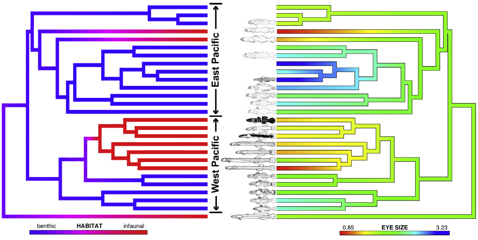
I just learned of this recent article by Ryan Ellingson et al. which makes very neat use of the phytools functions densityMap and contMap for plotting a posterior density from stochastic mapping on a tree, and for mapping a continuous character on the tree (respectively). See Revell (2013) for more details. Below is a reproduction of their figure. On the left is a posterior density from stochastic mapping of 'benthic' vs. 'infaunal' habit; whereas on the right is a projection of the observed or reconstructed values of a continuous character, relative eye size. For more details see the original article, Ellingson et al. (2013).

Click here for larger version.

**Disclaimer: neither densityMap nor contMap can be used (directly) to add tiny line images of fishes to your tree!

Minor update to phyl.cca

A phytools user reported that phyl.cca breaks if either X or Y contain only one column. Even though we would not normally use CCA when one or the other of our xs or ys contains only one variable (why not use multivariable regression instead?) there is no theoretic reason why it should not work. The main reason seems to be R's different behavior towards vectors & matrices with one column.

The updated code is here. Please let me know if you run into any problems.

New OU simulator in fastBM

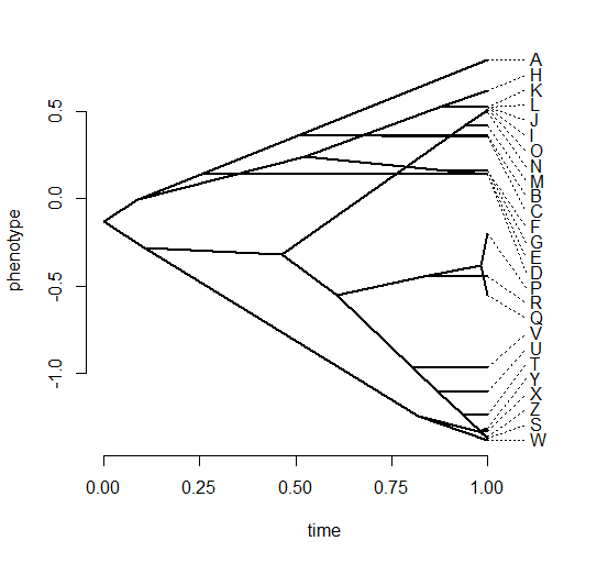
I just wrote some code for my phylogeny methods class (class materials here) to simulate evolution on the phylogeny by the Ornstein-Uhlenbeck process using a constant θ and α without transforming the tree. I think that what I did is correct. I have posted the code (it is an internally called function of fastBM) here. It is also in a minor phytools version (phytools 0.3-77) which can be downloaded & installed from source.

One of the main reasons it could be interesting to simulate OU using my function - rather than by first transforming the tree using transform.phylo (formerly ouTree) in the geiger package & then simulating on the transformed tree using BM - is because it can be used to simulate θ (the position of the optimum) that is different from the x₀, the state at the root node. As many of you probably know - it is not possible to fit this model to a tree with contemporaneous tips (the model is non-identifiable); however simulating under the model presents no problem theoretically.

Here's a quick demo:

> require(phytools)
Loading required package: phytools
> packageVersion("phytools")
[1] ‘0.3.77’
> tree<-pbtree(n=26,tip.label=LETTERS,scale=10)
> x<-fastBM(tree,a=0,theta=3,alpha=0.2,sig2=0.1, internal=TRUE)
> phenogram(tree,x,spread.labels=TRUE,spread.cost= c(1,0.01))

To create the plot above also requires a new version of phenogram, which handles label spreading slightly different (using the full range on the vertical axis, rather than simply the range of tip values for extant species). This is also in the latest phytools version.

Computing the posterior probabilities for tip nodes from ancThresh

The phytools function ancThresh, which conducts ancestral state reconstruction of a discrete character under the threshold model using Bayesian MCMC (Revell In press), also allows uncertain tip nodes in the tree. Uncertainty in the tip states are treated as a set of prior probability distributions on the states of terminal species in the tree. In this case, we can also compute posterior probabilities that each tip is in each state. These are automatically plotted by ancThresh if ancThresh(...,control=list(tipcol="estimated"). The burn-in that is used to compute these posterior probabilities is the user supplied burn-in in ancThresh(...,control=list(burnin)).

Unfortunately, and unlike the posterior probabilities for internal nodes, these probabilities are not returned to the user nor are they especially easy to compute. This is because the list component $mcmc only contains the implied states at internal nodes; and thus to get the posterior probabilities for tips, we need to use $liab and $par (which contains the sampled positions of the thresholds for each generation of the MCMC) to get the states.

Here is some code that can be used to compute these probabilities. In the example, mcmc is our object returned by ancThresh:

burnin<-200000 ## for instance
## find the row with the first post-burnin sample
ii<-which(mcmc$par[,"gen"]==burnin)
## number of tips
n<-length(tree$tip.label)
## states for the discrete character
states<-colnames(mcmc$par)[2:(ncol(mcmc$par)-1)]
## create and populate our matrix of posterior probabilities
PP<-matrix(NA,n,length(states),dimnames=
  list(colnames(mcmc$liab[1:n]),states))
for(i in 1:n){
  x<-vector(length=nrow(mcmc$liab)-ii+1)
  for(j in ii:nrow(mcmc$liab))
    x[j-ii+1]<-threshState(mcmc$liab[j,i],
      mcmc$par[j,2:(ncol(mcmc$par)-1)])
  PP[i,]<-summary(factor(x,levels=states))/length(x)
}

That's it.

S3 methods for phyl.pca

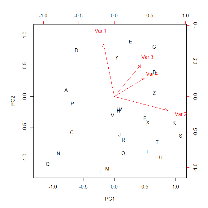
This morning Joan Maspons kindly supplied code for several S3 methods that can be used with the phytools function phyl.pca to return results via print, summary, and biplot that are similar to the equivalent S3 methods for objects of class prcomp. After a few minor tweaks (source code here) I have added these methods to the phytools package. The object returned by phyl.pca is in no way changed (it's merely been assigned the class attribute "phyl.pca"), so any prior functions designed to work with phyl.pca should still function. The updates are in a new minor phytools release phytools 0.3-74.

Here's a quick demo:

> library(phytools)
Loading required package: ape
Loading required package: maps
Loading required package: rgl
> packageVersion("phytools")
[1] ‘0.3.74’
> ## simulate tree
> tree<-pbtree(n=26,scale=1,tip.label=LETTERS)
> ## simulate data
> X<-fastBM(tree,nsim=4)
> ## phylogenetic PCA
> pca<-phyl.pca(tree,X,mode="cov")
> ## S3 print method
> pca
Phylogenetic pca
Starndard deviations:
      PC1       PC2       PC3       PC4
1.1851495 1.1200792 0.9641014 0.4812711
Loads:
            PC1        PC2         PC3        PC4
[1,] -0.1915766  0.9282404  0.15015897 -0.2812837
[2,]  0.9346040 -0.2431641 -0.03290792 -0.2574947
[3,]  0.4657425  0.5602278 -0.65456104  0.2019371
[4,]  0.5296652  0.3231947  0.74759143  0.2368691
> summary(pca)
Importance of components:
                         PC1   PC2   PC3   PC4
Standard deviation     1.185 1.120 0.964 0.481
Proportion of Variance 0.368 0.328 0.243 0.060
Cumulative Proportion  0.368 0.696 0.939 1.000
> biplot(pca)

Reconstructed ancestral & tip states for a continuous character evolving by Brownian motion with missing data

I'm working on a short comment (perhaps for publication, perhaps not) on ancestral state reconstruction methods when data for some tips are missing or uncertain. The reason for this is twofold: (1) enough people have asked me about this that it seems some kind of literature reference might be handy; and (2) little to no modification of existing approaches is required to reconstruct ancestral states when some tip states are uncertain or unknown. For instance, this is a routine matter in the reconstruction of ancestral DNA sequences when some tip states are ambiguous.

Possibly the least interesting case for reconstructing ancestral states when some of the data for tips are unknown is ML estimation of ancestral values of a continuous character under constant-rate Brownian motion. This is (1) because ML ancestral states for the parent nodes of lineages leading to tip taxa with missing are exactly the same as the states we'd obtain by linearly interpolating on the basis of the states at subtending nodes, and (2) because ML states for the missing tips in the tree are (under BM which has an expected change of zero with variance σ²t along any edge of length t, remember) identical to the reconstructed state at the parent node.

Uninteresting as it might be in most cases, we can nonetheless do this. I just modified the phytools function anc.ML to attempt this if some tips in the tree are missing from the data vector, x. Here's a simple demo to show what I mean:

> library(phytools)
> source("anc.ML.R")
> tree<-pbtree(n=26,scale=1,tip.label=LETTERS)
> yy<-x<-fastBM(tree)
> x<-sample(x,13)
> X<-anc.ML(tree,x)
> setdiff(names(yy),names(x))
 [1] "B" "D" "F" "J" "K" "L" "M" "N" "R" "T" "U" "V" "X"
> phenogram(tree,c(x,X$missing.x,X$ace),spread.labels=TRUE, spread.cost=c(1,0))

If you look closely at the list of missing taxa returned by setdiff and the plotted traitgram you'll see (just as promised) the reconstructed phenotypes of missing tips are connected to their ancestors (interpolated perfectly along the subtending branch) by precisely horizontal lines.

That's it.

New function to add species to a genus in a phylogeny

Recently an R-sig-phylo subscriber made the following request:

"I need to add a list of 230 species in a phylogenetic tree. Is there a logical way to add the species to the root of the genera to which it belongs, in a systematic way, that is, to make a function recognizes the name of the genera to which the species belongs, and so it adds the species to that root?"

I posted a solution to this, but I also thought that other phytools users might face the same problem so I have now automated this in the function add.species.to.genus. This, along with the matrix comparison function skewers, is also in a new minor phytools build (phytools 0.3-73).

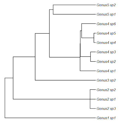
The function works by first peeling the genus name out of the species name. It does this by looking for either the underscore character, "_", or a space character, " ". It then proceeds to identify the clade containing con-generics in the tree by matching the genus name to the tip labels. Finally, it can either attach the new species to the root node of the most inclusive clade containing congenerics; or it can attach the new species randomly within that clade. In general, the function works best if the input tree is ultrametric. Otherwise, it may return a tree without edge lengths!

Here's a quick demo:

> ## load phytools
> library(phytools)
Loading required package: ape
Loading required package: maps
Loading required package: rgl
> packageVersion("phytools")
[1] ‘0.3.73’
> ## here's our starting tree
> plotTree(tree,ftype="i")

> ## add a species to 'Genus2' at root of genus
> species<-"Genus2_sp3"
> t1<-add.species.to.genus(tree,species)
> plotTree(t1,ftype="i")

> ## add a species to 'Genus4' randomly in genus
> species<-"Genus4 sp7"
> t2<-add.species.to.genus(tree,species,where="random")
> plotTree(t2,ftype="i")

> ## add a set of species in a vector
> species<-c("Genus1_sp2", "Genus2_sp3", "Genus3_sp2", "Genus4_sp7", "Genus4_sp8", "Genus5_sp3")
> for(i in 1:length(species)) tree<-add.species.to.genus(tree,species[i],where="random")
> plotTree(tree,ftype="i")

If the user supplies a species name for a genus with only one representative in the tree; a species with no congeners in the tree; or a genus that is non-monophyletic, in each case the function will try to do something rational and return a warning.

That's it.

Random skewers method for comparing covariance matrices

A colleague and friend emailed me the other day to ask me if I had any R code for the so-called "random skewers" matrix comparison method of Cheverud (1996). According to this method, we 'skewer' our target pair of covariance matrices with a set of random selection vectors and then measure the (vector) correlation between the response. The strength of this correlation (compared to the correlation of random vectors) is a measure of the similarity of our matrices. The method is perhaps most clearly described in Cheverud & Marroig (2007).

Well, I don't have code - but it was relatively easy to come up with. The biggest challenge is trying to figure out where the null distribution for the correlation comes from. In Cheverud & Marroig (2007) they suggest that we can just generate random vectors where the elements come from a uniform distribution & then compute the correlations between these random vectors. In my limited trials, though, this seems to result in elevated type I error. Alternatively, perhaps we should generate pairs of random covariance matrices using some model, and then compute the mean correlation between random vectors used to skewer our random covariance matrices. If the model for our covariance matrices is the same one used to generate our null distribution, then we seem to end up with type I error at or around the nominal level; as well as p-values more or less uniform on the interval [0, 1], which is another good sign. Unfortunately, this method is much more computationally intensive.

I've posted code for this function on the phytools page here. It depends on clusterGeneration, so this should be installed before attempting to run the code!

Let's try it using genPositiveDefMat(...,covMehod="unifcorrmat") for our covariance matrix & null hypothesis test:

> source("skewers.R")
> library(clusterGeneration)
> foo<-function(){
X1<-genPositiveDefMat(dim=5,covMethod="unifcorrmat")$Sigma
X2<-genPositiveDefMat(dim=5,covMethod="unifcorrmat")$Sigma
skewers(X1,X2,nsim=100,method="unifcorrmat")
}
> X<-replicate(200,foo(),simplify=TRUE)
> mean(unlist(X["p",])<=0.05)
[1] 0.065
> hist(unlist(X["p",]),main="histogram of p",xlab="p", col="grey")

Now let's try it for simulated empirical VCV matrices that are derived from data simulated using the same underlying covariance structure:

> library(mnormt)
> V<-genPositiveDefMat(dim=5,covMethod="unifcorrmat")$Sigma
> X<-rmnorm(n=30,varcov=V)
> Y<-rmnorm(n=30,varcov=V)
> X<-cov(X)
> Y<-cov(Y)
> skewers(X,Y,method="unifcorrmat")
$r
[1] 0.9397734
$p
[1] 0

This is offered without any guarantees. Please let me know if you find any errors.