A colleague asked me today if it was possible to run brownie.lite() on an arbitrarily specified set of rate regimes, rather than on the set of regimes obtained by mapping a discrete character on the phylogeny (say, using the technique of stochastic character mapping; Huelsenbeck et al. 2003). The simpler answer is "yes" - but it is a tiny bit complicated. brownie.lite() still needs a modified "phylo" object, as created by read.simmap() or make.simmap(), but we can actually build that object ourselves without too much difficulty.
To understand how to do this, we should recall the structure of the simmap "phylo" object in memory. I have blogged about this previously (e.g., here). The modified object contains two additional elements: $mapped.edge, which is a matrix containing the total time spent in each state on each edge, and $maps, which contains both the times and sequences of states on each edge. brownie.lite() uses only $mapped.edge, so we should focus on that.
Let's first consider the simplest case in which each branch, and no fractions of branches, are assigned to specific rate regimes. Say we have a list of branches in each state, where branches are indicated by the node numbers with which these end. Node numbers are the numbers given in the "phylo" object element $edge. For this example, let's say the branches in state "0" are contained in nodes0 and the branches in state "1" in nodes1. Our phylogenetic tree is tree.
First, create the element mapped.edge:
> tree$mapped.edge<-matrix(0,nrow(tree$edge),2, dimnames=list(edge=apply(tree$edge,1,function(x) paste(x,collapse=",")),state=c("0","1")))
Now fill in the matrix:
> tree$mapped.edge[match(nodes0,tree$edge[,2]),"0"]<- tree$edge.length[match(nodes0,tree$edge[,2])]
> tree$mapped.edge[match(nodes1,tree$edge[,2]),"1"]<- tree$edge.length[match(nodes1,tree$edge[,2])]
That's it. Now we have an object, tree, suitable for brownie.lite().
Wednesday, July 27, 2011
Monday, July 18, 2011
Updates to plotTree() and plotSimmap(); new phylogenetics movie
I just fixed a bug in plotTree(). It is the same bug as was described for plotSimmap() here (and solved). The new version of this function can be downloaded from my R phylogenetics page (direct link to code here).
I also added the option to plot no tip labels in plotSimmap(). This is accomplished by setting ftype="off". Code here.
Finally, I just spotted a poster for what I can only assume is a movie about phylogenetics. I snapped a photo on my smartphone:

Coming soon to a theater near you!
I also added the option to plot no tip labels in plotSimmap(). This is accomplished by setting ftype="off". Code here.
Finally, I just spotted a poster for what I can only assume is a movie about phylogenetics. I snapped a photo on my smartphone:

Coming soon to a theater near you!
Friday, July 15, 2011
New function: map.overlap()
I just posted a new function that comes from a project I am currently working on. This function computes the fractional overlap between the mapped states of two different stochastic mapped trees. I will try to describe the algorithm that I used for this in a subsequent post (since I think it is pretty neat), but first, I thought I'd illustrate use of the function first.
First, load "phytools" and the function from source (direct link to source code for function here):
> require(phytools)
> source("map.overlap.R")
Now, let's read in a pair of simmap trees:
> tree1<-read.simmap(text="((((3:{1,0.2442},4:{1,0.2442}):{1,0.4139},2:{1,0.0207:2,0.6374}):{1,0.3572},5:{1,0.4678:2,0.3717:1,0.053:2,0.1227}):{1,0.4471},1:{1,0.4228:2,0.2277:1,0.0564:2,0.7554});")
> tree2<-read.simmap(text="((((3:{1,0.2442},4:{1,0.2442}):{1,0.4139},2:{1,0.0214:2,0.6367}):{1,0.3572},5:{1,0.6239:2,0.3914}):{1,0.0034:2,0.2051:1,0.0511:2,0.1639:1,0.0237},1:{1,0.963:2,0.4993});")
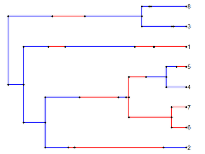
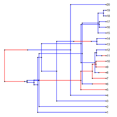
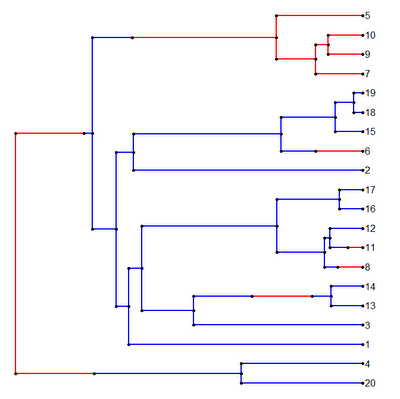
Below is a plot of these trees created using plotSimmap(), but in which I have overlayed the graphs so that they can be more easily compared. (Remember, the colors of the vertical branches are meaningless.)
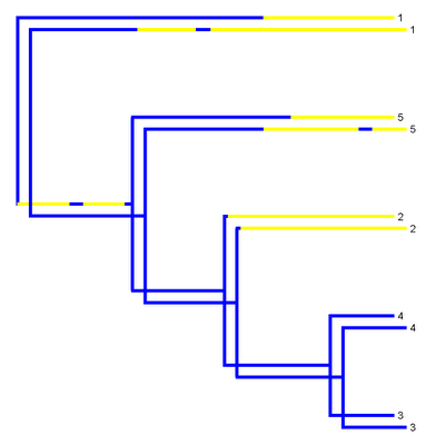
Because the rate of evolution in the mapped character trait is low (and, thus, the character doesn't change very much), the overlap between the two different stochastic maps seems high. Let's compute its precise value using my function map.overlap():
> map.overlap(tree1,tree2,tol=1e-3)
[1] 0.7805543
We need to set the tolerance level quite high here because I have rounded the mapped edge lengths so that the Newick string for the tree doesn't fill up this blog window!
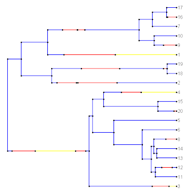
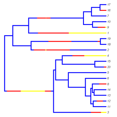
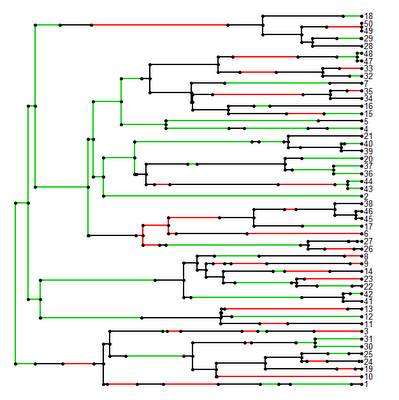
Now, for comparison, let's consider two simmap trees where the mapped state changes much more frequently (I won't give the Newick strings because they are far too long):
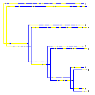
> map.overlap(tree3,tree4,tol=1e-3)
[1] 0.5369969
The overlap is much lower, just as we'd expect. Cool.
First, load "phytools" and the function from source (direct link to source code for function here):
> require(phytools)
> source("map.overlap.R")
Now, let's read in a pair of simmap trees:
> tree1<-read.simmap(text="((((3:{1,0.2442},4:{1,0.2442}):{1,0.4139},2:{1,0.0207:2,0.6374}):{1,0.3572},5:{1,0.4678:2,0.3717:1,0.053:2,0.1227}):{1,0.4471},1:{1,0.4228:2,0.2277:1,0.0564:2,0.7554});")
> tree2<-read.simmap(text="((((3:{1,0.2442},4:{1,0.2442}):{1,0.4139},2:{1,0.0214:2,0.6367}):{1,0.3572},5:{1,0.6239:2,0.3914}):{1,0.0034:2,0.2051:1,0.0511:2,0.1639:1,0.0237},1:{1,0.963:2,0.4993});")
Below is a plot of these trees created using plotSimmap(), but in which I have overlayed the graphs so that they can be more easily compared. (Remember, the colors of the vertical branches are meaningless.)

Because the rate of evolution in the mapped character trait is low (and, thus, the character doesn't change very much), the overlap between the two different stochastic maps seems high. Let's compute its precise value using my function map.overlap():
> map.overlap(tree1,tree2,tol=1e-3)
[1] 0.7805543
We need to set the tolerance level quite high here because I have rounded the mapped edge lengths so that the Newick string for the tree doesn't fill up this blog window!
Now, for comparison, let's consider two simmap trees where the mapped state changes much more frequently (I won't give the Newick strings because they are far too long):

> map.overlap(tree3,tree4,tol=1e-3)
[1] 0.5369969
The overlap is much lower, just as we'd expect. Cool.
More robust version of brownie.lite()
I just posted a slightly more robust version of brownie.lite(), a function that implements the method of O'Meara et al. (2006).
In the previous versions, the "stats" general purpose optimizer, optim(), would occasionally (say, 1 in 100 times) falsely converge - that is, converge for the multi-rate model to a region of parameter space that is far from the true optimum and had a very low likelihood - but nonetheless believe that it had found the maximum of the likelihood surface. Oops! This is not a huge problem because when this happens it usually results in a multi-rate model likelihood that is much worse than the likelihood of the single-rate model. (By definition, this is impossible since the models are nested.) The difference in the log-likelihoods between the simpler one-rate model and the more complex multi-rate model in this case can be huge (for instance -177.58 compared to -4776.32 in one example), and thus we can easily see that we have had a problem with optimizing the multi-rate model.
To avoid this kind of gross non-convergence, I have now added a while() loop in which I check to ensure that the multi-rate model has at least as good a likelihood as the one-rate model, and re-optimize the model with different random starting values while it does not:
while(logL2 < logL1){
message("False convergence on first try; trying again with new starting values.")
model2<-optim(starting*2*runif(n=length(starting)), fn=likelihood.multiple,y=x,C=C2,control=list(maxit=maxit), hessian=TRUE,method="L-BFGS-B",lower=lower)
logL2<--model2$value
}
Anyway, this seems to help. Other non-convergence can probably be fixed by increasing maxit in the function arguments, e.g.:
> brownie.lite(...,maxit=4000) # default is 2000
Good luck!
Thursday, July 14, 2011
Updates and new version of "phytools" (v0.0-5)
I just posted a new version of the "phytools" package (here), v0.0-5. This version contains a few different updates.
1) I renamed the function min.split() to minSplit() and the function split.tree() to splitTree() to resolve generic/method inconsistencies. This is because R has generic functions min and split, but my functions don't comply with these generic methods. The renaming of splitTree() should not cause users any trouble, as this is called only from within posterior.evolrate(). Description of the use of min.split() can be found here and here; minSplit() works exactly the same way.
2) write.simmap() now writes to file in addition to a text string. It still only accepts modified "phylo" objects, and not "multiPhylo" lists of simmap trees; but allows for append=TRUE, which means that multiple simmap trees can be printed to file using a simple for() loop.
For instance:
> require(geiger)
> require(phytools)
> tree<-birthdeath.tree(b=1,d=0,taxa.stop=100)
> x<-sim.char(tree,model.matrix=list(matrix(c(-1,1,1,-1),2,2)), model="discrete")[,,1]
> mtrees<-make.simmap(tree,x,nsim=100)
> for(i in 1:length(mtrees)) write.simmap(mtrees[[i]],"testfile.trees",append=T)
3) Finally, I created a generic help page for "phytools":
> require(phytools)
> ?phytools
Good luck - and please post feedback if you try this version.
Wednesday, July 13, 2011
Update to make.simmap() to generate multiple maps
Obviously, the purpose of stochastic character mapping is to sample possible character histories with according to their posterior probability (Huelsenbeck et al. 2003). With the previous version of make.simmap() it was only possible to do this by running the function many times with the same data and tree. This involved the totally unnecessary inefficiency of repeatedly calculating the conditional likelihoods using the "ape" function ace(). This is actually the slowest part of make.simmap() by a wide margin, e.g.:
> system.time(mtree<-make.simmap(tree,x))
user system elapsed
0.49 0.00 0.50
> system.time(XX<-ace(x,tree,type="discrete",model="SYM"))
user system elapsed
0.32 0.00 0.32
Since these likelihoods are the same each time we run make.simmap() (that is, for a given tree, data vector, and model), we should not recalculate them for every stochastic map that we want to simulate. In the latest version of make.simmap(), which I have just posted online (here), we just calculate the conditional likelihoods once - and then we use them for each simulation on the tree. This prevents computation time from rising linearly with the number of simulated maps that we want. For instance, let's use "geiger" to simulate a tree and data; and then the new version of make.simmap() to simulate on the tree:
> require(geiger)
> tree<-drop.tip(birthdeath.tree(b=1,d=0,taxa.stop=101),"101")
> x<-sim.char(tree,model.matrix=list(matrix(c(-1,1,1,-1),2,2)), model="discrete")[,,1]
> system.time(mtree.single<-make.simmap(tree,x))
user system elapsed
0.52 0.00 0.52
> system.time(mtree.multiple<-make.simmap(tree,x,nsim=100))
user system elapsed
19.69 0.00 19.69
So, not super fast, but better (by 30s over 100 replicates) than had we just looped the old version of make.simmap() 100 times.
Monday, July 11, 2011
Writing a "simmap" tree to file
Ok, I just completed a very basic function to write a stochastic character mapped tree to file. The function is built on the general (if somewhat inelegant) algorithm for writing a "phylo" object to a Newick string that I gave in a previous post. This function is available from my R phylogenetics page (direct link to code here) and it will eventually join the "phytools" package.
Here's a quick example of potential usage. Let's start with our Newick tree from before:
> tree<-read.tree(text="(((2:1.55,((6:0.16,7:0.16):0.47,(4:0.22,5:0.22):0.41):0.92):0.24,1:1.79):0.17,(3:0.49,8:0.49):1.47);")
Now, let's simulate a discrete character on this tree using sim.char() from the "geiger" package:
> require(geiger)
> x<-sim.char(tree,model.matrix=list(matrix(c(-1,1,1,-1),2,2)), model="discrete")[,,1]
> x
2 6 7 4 5 1 3 8
1 2 2 1 2 2 1 1
Next, we can use make.simmap() to simulate a stochastic character map:
> mtree<-make.simmap(tree,x)
And we can plot it:
> cols<-c("blue","red"); names(cols)<-c(1,2)
> plotSimmap(mtree,cols,lwd=3,pts=F)
Finally, let's write the tree to a string:
> write.simmap(mtree)
[1] "(((2:{1,1.55},((6:{2,0.16},7:{2,0.16}):{1,0.01292597:2,0.13960021:1,0.22833548:2,0.08913835},(4:{1,0.22},5:{1,0.21640896:2,0.00359104}):{1,0.41}):{1,0.92}):{1,0.24},1:{1,0.0532546:2,0.59924269:1,0.1929242:2,0.94457851}):{1,0.17},(3:{1,0.24224632:2,0.09203948:1,0.15571419},8:{1,0.49}):{1,0.17465378:2,0.4633267:1,0.13014025:2,0.64147628:1,0.060403});"
Obviously, we can also write this to file. It is not built into write.simmap() yet, but we can just do:
> write(file="treefile.tre",write.simmap(mtree))
Or multiple trees:
> write(file="treefile.tre",write.simmap(make.simmap(tree,x)))
> write(file="treefile.tre",write.simmap(make.simmap(tree,x)), append=T)
Which we can then, of course, read in using read.simmap():
> trees<-read.simmap("treefile.tre")
Read 2 items
> plotSimmap(trees[[1]],cols)
> plotSimmap(trees[[2]],cols)
Cool!
Here's a quick example of potential usage. Let's start with our Newick tree from before:
> tree<-read.tree(text="(((2:1.55,((6:0.16,7:0.16):0.47,(4:0.22,5:0.22):0.41):0.92):0.24,1:1.79):0.17,(3:0.49,8:0.49):1.47);")
Now, let's simulate a discrete character on this tree using sim.char() from the "geiger" package:
> require(geiger)
> x<-sim.char(tree,model.matrix=list(matrix(c(-1,1,1,-1),2,2)), model="discrete")[,,1]
> x
2 6 7 4 5 1 3 8
1 2 2 1 2 2 1 1
Next, we can use make.simmap() to simulate a stochastic character map:
> mtree<-make.simmap(tree,x)
And we can plot it:
> cols<-c("blue","red"); names(cols)<-c(1,2)
> plotSimmap(mtree,cols,lwd=3,pts=F)

Finally, let's write the tree to a string:
> write.simmap(mtree)
[1] "(((2:{1,1.55},((6:{2,0.16},7:{2,0.16}):{1,0.01292597:2,0.13960021:1,0.22833548:2,0.08913835},(4:{1,0.22},5:{1,0.21640896:2,0.00359104}):{1,0.41}):{1,0.92}):{1,0.24},1:{1,0.0532546:2,0.59924269:1,0.1929242:2,0.94457851}):{1,0.17},(3:{1,0.24224632:2,0.09203948:1,0.15571419},8:{1,0.49}):{1,0.17465378:2,0.4633267:1,0.13014025:2,0.64147628:1,0.060403});"
Obviously, we can also write this to file. It is not built into write.simmap() yet, but we can just do:
> write(file="treefile.tre",write.simmap(mtree))
Or multiple trees:
> write(file="treefile.tre",write.simmap(make.simmap(tree,x)))
> write(file="treefile.tre",write.simmap(make.simmap(tree,x)), append=T)
Which we can then, of course, read in using read.simmap():
> trees<-read.simmap("treefile.tre")
Read 2 items
> plotSimmap(trees[[1]],cols)
> plotSimmap(trees[[2]],cols)


Cool!
Writing a "phylo" object to a Newick string
Now that we can generate stochastic character mapped trees using make.simmap(), I thought it would be useful to write them to file. Unfortunately, although I have functions that can read Newick strings from file (e.g., read.newick() and read.simmap()), I don't yet have code to go the other way (i.e., to write a Newick string from a "phylo" object stored in memory). For more details on the Newick convention, check out Felsenstein's comprehensive description.
Ok, now, remember how a "phylo" object is stored. It is a list with three essential components: $edge, a matrix containing the node or tip numbers for the upper and lower node of each edge; $tip.label, a vector containing the labels for each tip; and, finally, $Nnode, an integer value indicating the number of internal nodes in the tree. Branch lengths are stored in the optional vector $edge.length, which contains all the branch lengths in tree tree in the order of $edge.
So, for instance, the Newick tree:
(((2:1.55,((6:0.16,7:0.16):0.47,(4:0.22,5:0.22):0.41):0.92):0.24,1:1.79):0.17,(3:0.49,8:0.49):1.47);
is plotted as follows:
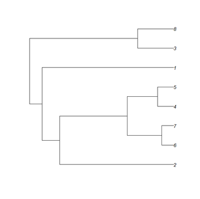
and is represented in memory with the following four parts:
> tree$edge
[,1] [,2]
[1,] 9 10
[2,] 10 11
[3,] 11 1
[4,] 11 12
[5,] 12 13
[6,] 13 2
[7,] 13 3
[8,] 12 14
[9,] 14 4
[10,] 14 5
[11,] 10 6
[12,] 9 15
[13,] 15 7
[14,] 15 8
> tree$tip.label
[1] "2" "6" "7" "4" "5" "1" "3" "8"
> tree$Nnode
[1] 7
> tree$edge.length
[1] 0.17 0.24 1.55 0.92 0.47 0.16 0.16 0.41 0.22 0.22 1.79 1.47 0.49 0.49
The task of back-translating the object above to a Newick string is not too difficult. In fact, if the "phylo" object is in "cladewise" order (as above), then we can nearly just descend from the top to the bottom of the matrix $edge, writing the appropriate characters at each step. The reason I qualify this as nearly is because we can move up (i.e., from root to tip) the tree very easily by descending $edge, we do not as easily move back down the tree this way - which we need to do to close parentheses and assign branch lengths to internal edges of the Newick tree. To do this, we just need to write a simple while() loop which backs down the tree every time we might be ready to close out a clade.
The code for my simple tree writer is not particularly elegant, but it seems to work:
writeTree<-function(tree){
tree<-reorder.phylo(tree,"cladewise")
n<-length(tree$tip)
string<-vector(); string[1]<-"("; j<-2
for(i in 1:nrow(tree$edge)){
if(tree$edge[i,2]<=n){
string[j]<-tree$tip.label[tree$edge[i,2]]; j<-j+1
if(!is.null(tree$edge.length)){
string[j]<-paste(c(":",round(tree$edge.length[i],10)), collapse="")
j<-j+1
}
v<-which(tree$edge[,1]==tree$edge[i,1]); k<-i
while(length(v)>0&&k==v[length(v)]){
string[j]<-")"; j<-j+1
w<-which(tree$edge[,2]==tree$edge[k,1])
if(!is.null(tree$edge.length)){
string[j]<-paste(c(":",round(tree$edge.length[w],10)), collapse="")
j<-j+1
}
v<-which(tree$edge[,1]==tree$edge[w,1]); k<-w
}
string[j]<-","; j<-j+1
} else if(tree$edge[i,2]>=n){
string[j]<-"("; j<-j+1
}
}
if(is.null(tree$edge.length)) string<-c(string[1:(length(string)-1)], ";")
else string<-c(string[1:(length(string)-2)],";")
string<-paste(string,collapse="")
return(string)
}
Now, let's test it out against "ape"'s write.tree() for a random tree:
> tree<-rtree(n=100)
> tree$edge.length<-round(tree$edge.length,6) # to avoid precision differences
> write.tree(tree)==writeTree(tree)
[1] TRUE
Cool! Now we're ready to handle printing "simmap" trees.
Saturday, July 9, 2011
New plotting options in plotSimmap()
Last night I added a few new simple plotting options to the function plotSimmap(). These don't require much explanation, and include ftype (options "reg", the default, "i", "b", and "bi"); lwd, an integer the line width for edges in the tree; and pts, a logical value indicating whether or not to plot filled circles at all vertices of the tree and at state transitions.
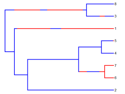
To see how these options can be used, lets first plot using the default values. The current tree has a three state mapped character, with states 1, 2, and 3.
> cols<-c("blue","yellow","red"); names(cols)<-c(1,2,3)
> plotSimmap(mtree,cols)
The first line is to create a vector with the colors we want; and the second line plots the tree. We get:
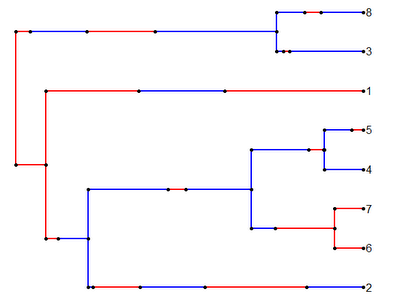
Now, let's get rid of the circles and plot the lines a little bit more thickly. (This is more like what we'd see if we used FigTree, for instance.) We can change the font to italics as well if we want:
> plotSimmap(mtree,cols,lwd=5,pts=F,ftype="i")
Now we get:
Updates are in the newest version (v0.4) of this function as well in the latest alpha version of the "phytools" package (available here)
To see how these options can be used, lets first plot using the default values. The current tree has a three state mapped character, with states 1, 2, and 3.
> cols<-c("blue","yellow","red"); names(cols)<-c(1,2,3)
> plotSimmap(mtree,cols)
The first line is to create a vector with the colors we want; and the second line plots the tree. We get:

Now, let's get rid of the circles and plot the lines a little bit more thickly. (This is more like what we'd see if we used FigTree, for instance.) We can change the font to italics as well if we want:
> plotSimmap(mtree,cols,lwd=5,pts=F,ftype="i")
Now we get:

Updates are in the newest version (v0.4) of this function as well in the latest alpha version of the "phytools" package (available here)
New version of "phytools"
I just posted a new alpha version (version 0.0-4) of the "phytools" package to my R-phylogenetics page, here. This version includes the function treeSlice(), as well as improvements and bug fixes to brownie.lite(), make.simmap(), and plotSimmap(). I will describe the new plotting options for plotSimmap() in a subsequent post.
Friday, July 8, 2011
Bug fix in plotSimmap()
Rafael Maia has identified an error in plotSimmap() that sometimes results in plotted trees that look like this:
Yikes!
The error is most easily replicated with the following example. Let's take this simple Newick style tree containing 8 taxa:
(((2:1.55,((6:0.16,7:0.16):0.47,(4:0.22,5:0.22):0.41):0.92):0.24,1:1.79):0.17,(3:0.49,8:0.49):1.47);
If we read this tree into memory using read.tree(), then the tips of the tree will be numbered from left to right in the Newick tree, i.e.:
> tree$edge
[,1] [,2]
[1,] 9 10
[2,] 10 11
[3,] 11 1
[4,] 11 12
[5,] 12 13
[6,] 13 2
[7,] 13 3
[8,] 12 14
[9,] 14 4
[10,] 14 5
[11,] 10 6
[12,] 9 15
[13,] 15 7
[14,] 15 8
> tree$tip.label
[1] "2" "6" "7" "4" "5" "1" "3" "8"
I naively assumed that this would always be true for trees in "cladewise" order, but in fact this is not the case. Let's read the same tree from "Nexus" format, which in this case might look something like this:
#NEXUS
BEGIN TAXA;
DIMENSIONS NTAX = 8;
TAXLABELS
1
2
3
4
5
6
7
8
;
END;
BEGIN TREES;
TRANSLATE
1 1,
2 2,
3 3,
4 4,
5 5,
6 6,
7 7,
8 8
;
TREE *, UNTITLED = [&R] (((2:1.55,((6:0.16,7:0.16):0.47,(4:0.22,5:0.22):0.41):0.92):0.24,1:1.79):0.17,(3:0.49,8:0.49):1.47);
END;
If we read this file in using read.nexus(), we end up with tips that are numbered according to the translation table - not the left-right order in the Newick string, i.e.,
> tree$edge
[,1] [,2]
[1,] 9 10
[2,] 10 11
[3,] 11 2
[4,] 11 12
[5,] 12 13
[6,] 13 6
[7,] 13 7
[8,] 12 14
[9,] 14 4
[10,] 14 5
[11,] 10 1
[12,] 9 15
[13,] 15 3
[14,] 15 8
> tree$tip.label
[1] "1" "2" "3" "4" "5" "6" "7" "8"
The issue with plotting arises because I assumed that the tip numbers were numerically ordered according the left-to-right order of the Newick string and simply evenly spaced the tips on the basis of this numerical order (which results in branch crossing when the tips are not ordered this way, as evidenced by the figure above). Luckily, this was not difficult to solve. I merely changed the line of code in which I assigned vertical coordinates to all the tips from:
Y[1:n]<-1:n
to:
Y[cw$edge[cw$edge[,2]<=length(cw$tip),2]]<-1:n
which seems to do the trick, as if we replot the tree above, our branch crossing is solved:
I have posted the fixed version on my R phylogenetics page (direct link to code here) and I will incorporate this into the next alpha release of "phytools."

Yikes!
The error is most easily replicated with the following example. Let's take this simple Newick style tree containing 8 taxa:
(((2:1.55,((6:0.16,7:0.16):0.47,(4:0.22,5:0.22):0.41):0.92):0.24,1:1.79):0.17,(3:0.49,8:0.49):1.47);
If we read this tree into memory using read.tree(), then the tips of the tree will be numbered from left to right in the Newick tree, i.e.:
> tree$edge
[,1] [,2]
[1,] 9 10
[2,] 10 11
[3,] 11 1
[4,] 11 12
[5,] 12 13
[6,] 13 2
[7,] 13 3
[8,] 12 14
[9,] 14 4
[10,] 14 5
[11,] 10 6
[12,] 9 15
[13,] 15 7
[14,] 15 8
> tree$tip.label
[1] "2" "6" "7" "4" "5" "1" "3" "8"
I naively assumed that this would always be true for trees in "cladewise" order, but in fact this is not the case. Let's read the same tree from "Nexus" format, which in this case might look something like this:
#NEXUS
BEGIN TAXA;
DIMENSIONS NTAX = 8;
TAXLABELS
1
2
3
4
5
6
7
8
;
END;
BEGIN TREES;
TRANSLATE
1 1,
2 2,
3 3,
4 4,
5 5,
6 6,
7 7,
8 8
;
TREE *, UNTITLED = [&R] (((2:1.55,((6:0.16,7:0.16):0.47,(4:0.22,5:0.22):0.41):0.92):0.24,1:1.79):0.17,(3:0.49,8:0.49):1.47);
END;
If we read this file in using read.nexus(), we end up with tips that are numbered according to the translation table - not the left-right order in the Newick string, i.e.,
> tree$edge
[,1] [,2]
[1,] 9 10
[2,] 10 11
[3,] 11 2
[4,] 11 12
[5,] 12 13
[6,] 13 6
[7,] 13 7
[8,] 12 14
[9,] 14 4
[10,] 14 5
[11,] 10 1
[12,] 9 15
[13,] 15 3
[14,] 15 8
> tree$tip.label
[1] "1" "2" "3" "4" "5" "6" "7" "8"
The issue with plotting arises because I assumed that the tip numbers were numerically ordered according the left-to-right order of the Newick string and simply evenly spaced the tips on the basis of this numerical order (which results in branch crossing when the tips are not ordered this way, as evidenced by the figure above). Luckily, this was not difficult to solve. I merely changed the line of code in which I assigned vertical coordinates to all the tips from:
Y[1:n]<-1:n
to:
Y[cw$edge[cw$edge[,2]<=length(cw$tip),2]]<-1:n
which seems to do the trick, as if we replot the tree above, our branch crossing is solved:

I have posted the fixed version on my R phylogenetics page (direct link to code here) and I will incorporate this into the next alpha release of "phytools."
Friday, July 1, 2011
Null distribution by simulation for brownie.lite()
I just posted a new version of brownie.lite() on my R-phylogenetics page (direct link to code here). Just to remind you, this function implements the non-censored evolutionary rates test of O'Meara et al. (2006). In the method we fit two different models using the technique of maximum likelihood - one in which one evolutionary rate prevails, and another in which the evolutionary rate shifts one or multiple times between two or more evolutionary rates on different branches of the tree. We can then compare the fit of these models by, for instance, comparing 2 × their log-likelihood ratio to a Χ2-distribution.
We could also compare the likelihood ratio to likelihood ratios obtained by simulating under the null hypothesis. (In fact, I believe that the authors suggested this in their original paper.) I have now implemented this test in brownie.lite(). I am also presently conducting a mini-experiment to compare the type I error rates of each method. Since the likelihood ratio is only asymptotically Χ2-distributed for large n, we might expect that the simulation test would be more conservative than the Χ2 test. So far I have not found a lot of evidence to suggest that it is for n=10 and n=20.
I'll also confess to a small fudge in the implementation of this method. Occasionally (i.e., about 1% of the time or so), brownie.lite() fails to converge during optimization. Rather than fix this, to avoid this problem when trying to compute the P-value by simulation, I just discarded any simulated datasets that were troublesome to optimize. I don't see how this would result in any bias, but I don't know. In the near future, I will fix this problem in brownie.lite() (and hopefully clean up the function in general, as it is pretty messy).
If you'd like to participate in my mini experiment, I encourage you to download the new version of brownie.lite() and try and run the following code (hopefully increasing nrep and varying nsp. Please post the results.
require(phytools)
require(geiger)
source("brownie.lite.R") # load new version of brownie.lite()
typeI.x2<-0; typeI.sim<-0
nrep<-100; nsp=20
for(i in 1:nrep){
# simulate tree
tree<-drop.tip(birthdeath.tree(b=1,d=0,taxa.stop=(nsp+1)), as.character(nsp+1))
# rescale tree
tree$edge.length<-tree$edge.length/mean(diag(vcv(tree)))
# simulate rate regime
x<-sim.char(tree,model.matrix=list(matrix(c(-1,1,1,-1),2,2)), model="discrete")[,,1]
while(length(unique(x))==1)
x<-sim.char(tree,model.matrix=list(matrix(c(-1,1,1,-1), 2,2)),model="discrete")[,,1]
mtree<-make.simmap(tree,x)
# simulate data under the null
y<-fastBM(tree)
# fit the model & compute X^2 P-value
result.x2<-brownie.lite(mtree,y,test="chisq")
# fit the model & compute simulation P-value
result.sim<-brownie.lite(mtree,y,test="simulation")
# count the frequence of P<0.05
typeI.x2<-typeI.x2+(result.x2$P.chisq<0.05)/nrep
typeI.sim<-typeI.sim+(result.sim$P.sim<0.05)/nrep
# something to look at while this is running
# (should converge to 0.05)
print(paste("X^2 type I error:",typeI.x2*nrep/i, "; Simulation type I error:",typeI.sim*nrep/i))
}
Small update to make.simmap()
I just posted a small update to my stochastic character mapping function, make.simmap(). The update fixes an error that arises when the tree has any edges that are exactly zero in length. Basically, the issue arose because I programmed the mapping along branch lengths as follows. For estimated transition matrix Q, I first set t to zero, and then I added random deviates from the exponential distribution with rate parameter -Qii (updating i for each state change in the character) while t is less than the total length of the current edge. Unfortunately, this does not work if the length of an edge is exactly zero. In addition, in this case there can be no change in state along the edge, and consequently we can just set our mapped state on that edge to be the sampled state at either the parent or daughter node (which our method of sampling node states guarantees will be the same).
The error in the previous version of make.simmap() will be revealed by the following code:
> require(phytools)
> require(geiger)
> tree<-birthdeath.tree(b=1,d=0,taxa.stop=50)
(birthdeath.tree(...,taxa.stop=N) stops the tree simulation at the moment that the Nth species appears, thus resulting in a pair of zero length terminal edges.)
> q<-list(matrix(c(-1,0.5,0.5,0.5,-1,0.5, 0.5,0.5,-1),3,3))
> x<-sim.char(tree,model.matrix=q,model="discrete")[,,1]
> mtree<-make.simmap(tree,x)
Error in if (names(map)[length(map)] == node.states[i, 2]) accept = TRUE :
argument is of length zero
However, if we load the new version of make.simmap(), the problem goes away:
> source("make.simmap.R")
> mtree<-make.simmap(tree,x)
> plotSimmap(mtree)
It works!
This updated version of make.simmap() will be in the next version of "phytools."
Of course, this does not deal with the issue of two taxa with zero evolutionary divergence that have different states. This will also cause an error in make.simmap() but this is more difficult to resolve because, in fact, two species with zero divergence should not have different phenotypes - and the probability that they do under our models will thus always be zero.
The error in the previous version of make.simmap() will be revealed by the following code:
> require(phytools)
> require(geiger)
> tree<-birthdeath.tree(b=1,d=0,taxa.stop=50)
(birthdeath.tree(...,taxa.stop=N) stops the tree simulation at the moment that the Nth species appears, thus resulting in a pair of zero length terminal edges.)
> q<-list(matrix(c(-1,0.5,0.5,0.5,-1,0.5, 0.5,0.5,-1),3,3))
> x<-sim.char(tree,model.matrix=q,model="discrete")[,,1]
> mtree<-make.simmap(tree,x)
Error in if (names(map)[length(map)] == node.states[i, 2]) accept = TRUE :
argument is of length zero
However, if we load the new version of make.simmap(), the problem goes away:
> source("make.simmap.R")
> mtree<-make.simmap(tree,x)
> plotSimmap(mtree)

It works!
This updated version of make.simmap() will be in the next version of "phytools."
Of course, this does not deal with the issue of two taxa with zero evolutionary divergence that have different states. This will also cause an error in make.simmap() but this is more difficult to resolve because, in fact, two species with zero divergence should not have different phenotypes - and the probability that they do under our models will thus always be zero.
Subscribe to:
Posts (Atom)