Friday, May 31, 2013

New CRAN version of phytools

There is a new version of phytools (phytools 0.2-80) now available on CRAN. It will probably take a few days for the Mac OS & Windows binaries to be compiled and to percolate through the mirror repositories.

Relative to the most recent CRAN build of phytools (phytools 0.2-70), this version has only a couple of significant updates, as follows:

1. A bug fix in make.simmap(..., type="mcmc"), described here.

2. The addition of the option to plot trees in a circular (type="fan") style to plotSimmap, plotTree, contMap, and densityMap (described here: 1, 2, 3, 4, 5, 6, 7, and 8).

Check it out.

Thursday, May 30, 2013

Bug fix in make.simmap(...,Q="mcmc")

I just posted a new version of make.simmap and a new phytools build (phytools 0.2-77). This version fixes a bug affecting make.simmap(...,Q="mcmc"). In this method, the transition matrix Q is sampled from its Bayesian posterior probability distribution using MCMC given the model & data. This sample is then used by make.simmap to map characters on the tree.

The bug was not in the MCMC itself which (so far as I can tell) is properly designed, but in how Q was stored in sampling generations - specifically, the updated value of Q for that generation was always stored. The reason this is not a bug in the MCMC is because this value was only returned to the chain with probability equal to the posterior odds ratio - thus this is only about the value that is stored from the chain, not the behavior of the chain itself. This was somewhat difficult to detect because it will not be obvious unless the variance on the proposal distribution is high relative to the curvature of the likelihood surface or the prior density. (In case it's not obvious why this is, this is because if the proposal variance is low - most post burn-in samples will have relatively high posterior odds and will thus have a good chance of being accepted; whereas if the proposal variance is high, most samples will have low posterior odds.)

I also changed the starting value of Q for the MCMC. Previously, I had arbitrarily set all the non-diagonal elements of Q to a fixed constant. Now I draw a set of values at random from the prior probability density on Q, as provided by the user. The advantage of this is because if we set a very strong prior on Q, our MCMC may have difficulty converging on the region of high posterior density if the variance on our proposal distribution is too low or (especially) high.

I'm not sure what a good proposal variance is - but one way of thinking about it is relative to the empirical Q. For instance, if the non-diagonal of our empirical Q are all around ~0.1, then it is probably not a good idea to vQ = 10. Unless our data contain very little information about Q, almost all samples will be rejected and the MCMC will be very inefficient at exploring the posterior distribution of Q. Conversely, if the non-diagonal of our empirical Q average > 100, then we should probably not choose vQ = 0.001. In this case, if we start anywhere near the ML of Q - and unless we have very little information about Q in our data - almost all samples will be accepted, which is also a bad way to sample from the posterior using MCMC.

Even though make.simmap is not set up for this, it is possible to do some diagnoses on our MCMC using the MCMC diagnostics package coda. For example, let's say we have obtained 100 samples of Q (and thus 100 stochastic mapped trees) from the posterior after burnin

mtrees<-make.simmap(tree,x,Q="mcmc",vQ=0.01,prior= list(use.empirical=TRUE,beta=2))
we can get the likelihoods using
logL<-sapply(unclass(mtrees),function(x) x$logL)
or (for instance), the posterior sample of Q1,2 using
q12<-sapply(unclass(mtrees),function(x) x$Q[1,2])
and then perform diagnostics (effective size, rejection rate, etc.) using the appropriate coda functions. To increase effective size without increasing the number of sampled trees, we can increase the sample frequency (samplefreq) and increase or decrease the proposal variance (vQ).

Monday, May 27, 2013

Circular trees in densityMap and contMap

In an earlier post I showed how plotSimmap(...,type="fan") could be used to plot densityMap or contMap style plots using the object of class "densityMap" or "contMap" returned invisibly by each function, respectively.

Well, I have now build this directly into contMap & densityMap (and the S3 generic plot for objects of class "densityMap" and "contMap"). Check it out:

> require(phytools)
Loading required package: phytools
> packageVersion("phytools")
[1] ‘0.2.76’
> contMap(tree,x,type="fan",fsize=0.9)
> X<-densityMap(mtrees,outline=TRUE,fsize=0.9)
sorry - this might take a while; please be patient

Argh - way too cluttered. Let's try a circular tree instead!

> class(X)
[1] "densityMap"
> plot(X,type="fan",fsize=0.9,outline=TRUE)

Since these updates involved changes to a number of methods in phytools - the best bet is to update to the latest non-CRAN phytools build (phytools 0.2-76).

That's it.

Sunday, May 26, 2013

Minor fixes to plotSimmap

I just fixed a couple of very minor issues with plotSimmap(...,type="fan"): specifically, lwd was not properly controlling the line width of edges; and ftype="off" (which should turn the labels off) was not working. The fixed function version of is here, along with a new minor phytools build (phytools 0.2-75).

We might want to turn off the labels if we have, for instance, a very large tree:

Click for larger version.

That's it for now.

Saturday, May 25, 2013

Some minor improvements to plotSimmap(...,type="fan") and a few other updates

I just posted a new version of plotSimmap and a new minor phytools version (phytools 0.2-74). The updates mainly do the following: (1) allows user control over close to the full range of plotting options in from plotSimmap(..., type="phylogram"); (2) change the shape of the line caps from round to square (to bring into alignment with plotSimmap(...,type="phylogram") and common sense); (3) improve the alignment of labels with the terminal edge their offset from the tips; and, finally, (4) fix some problems where not enough space was left around the plotted trees to allow the labels to be added (this also seems to affect plot.phylo(...,type="fan")).

The result looks very nice. Here's a quick demo using the phylogeny of 100 Greater Antillean anoles from Mahler et al. (2010) and a stochastic mapping of "ecomorph class" (including non-ecomorph species) on the tree. leg gives the color→ecomorph translation.

> require(phytools)
Loading required package: phytools
> packageVersion("phytools")
[1] ‘0.2.74’
> data(anoletree) # load tree
> states<-sort(unique(getStates(anoletree))) # get states
> # set color legend
> leg<-setNames(palette()[1:7],c(states[3],states[-3]))
> leg
Non-    CG    GB       TC     TG     Tr        TW
"black" "red" "green3" "blue" "cyan" "magenta" "yellow"
> # ok - here is a trick to plot an outline around the tree
> par(col="white")
> plotTree(anoletree,type="fan",lwd=4,mar=rep(0,4), fsize=0.8)

Note: type="fan" is in development.
Many options of type="phylogram" are not yet available.

> par(col="black")
> plotSimmap(anoletree,leg,type="fan",lwd=2,mar=rep(0,4), add=TRUE,fsize=0.8)

Note: type="fan" is in development.
Many options of type="phylogram" are not yet available.


(Click for highest resolution.)

Cool.

I also now allow type="fan" trees to be plotted from plotTree, which uses plotSimmap internally.

Friday, May 24, 2013

Raster image files from circular trees in R

There is some noticeable aliasing in circular (type="fan") trees exported directly from R in a raster format such as .png or .jpg. This can be overcome by exporting instead in a lossless vector format such as .pdf or .eps.

For example, here is a circular contMap style tree exported from R as a .png:

(Click for highest resolution version.)

Whereas here is the same tree exported as a .pdf, then read into Illustrator & exported as a much higher quality .jpg (a raster graphic format):

(Click for highest resolution version.)

Creating a type="fan" densityMap or contMap plot

I have not yet added the "type" argument to functions densityMap or contMap; however it is already possible to create a circular densityMap or contMap style tree. Here's how:

> require(phytools)
Loading required package: phytools
> packageVersion("phytools")
[1] ‘0.2.71’
> # simulate tree & data
> tree<-pbtree(n=100,scale=1)
> x<-fastBM(tree)
> # first plot typical contMap & obtain "contMap" object
> XX<-contMap(tree,x) # we don't care about this one
> # now plot with type="fan"
> plotSimmap(XX$tree,XX$cols,type="fan")
Note: type='fan' is in development. Most options not yet available.
> # finally, add color bar
> # (we have to click where we want this)
> add.color.bar(0.8,cols=XX$cols,title="trait value", lims=range(x),digits=2)

Note that we have to click where we want to put the color bar/legend.

That's it.

Thursday, May 23, 2013

New version of plotSimmap with type="fan"

Today I posted twice (1, 2) in response to Rafael Maia's early morning query about plotting stochastic mapped trees in a circular style. My earlier posts were about plotting the structure of a circular tree and adding a mapped discrete character using colors.

Well, all that was left was the labels. This is easier said that done. The first challenge was rotating the orientation of the labels to match the angle of their corresponding terminal edge. Here is my code to do that:

# plot labels
for(i in 1:n){
  ii<-which(cw$edge[,2]==i) # find edge
  aa<-Y[ii,2]/(2*pi)*360 # compute angle
  # fix angle & adjust to flip at 90 & 270 deg
  adj<-if(aa>90&&aa<270) c(1,0.5) else c(0,0.5)
  aa<-if(aa>90&&aa<270) 180+aa else aa
  # plot label
  text(x[ii,2],y[ii,2],cw$tip.label[i],srt=aa,adj=adj,
    cex=fsize)
}

The second challenge is making sure that we have a plotting window with enough space for our labels. For this, I stole a trick that I used in the function phenogram and described here.

Code for the new version of plotSimmap is here. I have also posted a new phytools version (phytools 0.2-71). Note that I have not applied all relevant options in plotSimmap to type="fan" yet. This will come in future.

For now - let's check out the version we have. Note that we need to first install the package plotrix.

> require(phytools)
Loading required package: phytools
> packageVersion("phytools")
[1] ‘0.2.71’
> tree<-pbtree(n=50,scale=2)
> Q<-matrix(c(-1,1,1,-1),2,2)
> rownames(Q)<-colnames(Q)<-letters[1:2]
> tree<-sim.history(tree,Q)
> cols<-setNames(c("blue","red"),letters[1:2])
> plotSimmap(tree,cols,type="fan")
Note: type='fan' is in development. Most options not yet available.

A miracle - it works!

Plotting a circular discrete character mapped tree, part II: The colors

Now that we've figured out how to plot the structure of a circular (i.e., "fan") tree, the next step is segmenting our plotted edges by a discrete character & then plotting segment by color. Here's my function for this next step. Note that (again) this depends on the package 'plotrix' and will not work if there is no character mapped on the tree:

plotFan<-function(tree,colors=NULL){
  if(!require(plotrix)) stop("install 'plotrix'")
  # check colors
  if(is.null(colors)){
    st<-sort(unique(unlist(sapply(tree$maps,names))))
    colors<-palette()[1:length(st)]
    names(colors)<-st
    if(length(st)>1){
      cat("no colors provided. ")
      cat("using the following legend:\n")
      print(colors)
    }
  }
  # reorder
  cw<-reorder(tree)
  pw<-reorder(tree,"pruningwise")
  # count nodes and tips
  n<-length(cw$tip)
  m<-cw$Nnode
  # get Y coordinates on uncurved space
  Y<-vector(length=m+n)
  Y[cw$edge[cw$edge[,2]<=length(cw$tip),2]]<-1:n
  nodes<-unique(pw$edge[,1])
  for(i in 1:m){
    desc<-pw$edge[which(pw$edge[,1]==nodes[i]),2]
    Y[nodes[i]]<-(min(Y[desc])+max(Y[desc]))/2
  }
  Y<-setNames(Y/max(Y)*2*pi,1:(n+m))
  Y<-cbind(Y[as.character(tree$edge[,2])],
    Y[as.character(tree$edge[,2])])
  R<-nodeHeights(cw)
  # now put into a circular coordinate system
  x<-R*cos(Y)
  y<-R*sin(Y)
  # plot nodes
  plot(x,y,axes=FALSE,asp=1)
  # plot radial lines (edges)
  for(i in 1:nrow(cw$edge)){
    maps<-cumsum(cw$maps[[i]])/sum(cw$maps[[i]])
    xx<-c(x[i,1],x[i,1]+(x[i,2]-x[i,1])*maps)
    yy<-c(y[i,1],y[i,1]+(y[i,2]-y[i,1])*maps)
    for(i in 1:(length(xx)-1))
      lines(xx[i+0:1],yy[i+0:1],
      col=colors[names(maps)[i]],lwd=2)
  }
  # plot circular lines
  for(i in 1:m+n){
    r<-R[match(i,cw$edge)]
    a1<-min(Y[which(cw$edge==i)])
    a2<-max(Y[which(cw$edge==i)])
    draw.arc(0,0,r,a1,a2,lwd=2,col=
      colors[names(cw$maps[[match(i,cw$edge[,1])]])[1]])
  }
}

The key attributes that I've added is segmentalization of each edge by the mapped state, and then separate plotting of each edge segment according to the colors for the state.

Let's try it out:

> Q<-matrix(c(-1,1,1,-1),2,2)
> rownames(Q)<-colnames(Q)<-letters[1:2]
> Q
   a  b
a -1  1
b  1 -1
> tree<-sim.history(tree,Q)
> plotSimmap(tree,colors=setNames(c("blue","red"), letters[1:2]))
> source("plotFan.R")
> plotFan(tree,colors=setNames(c("blue","red"), letters[1:2]))

Cool. Now we just need to clean it up a bit & add labels....

Plotting the structure of a circular ("fan") tree

Rafael Maia asks:

It would be really cool if simmap and densityMap trees could be plotted as radial (type='fan' in plot.phylo) trees. I find it much easier to visualize the patterns when the tree is quite large.

Indeed this would be quite cool. The first step is to figure out how to plot the structure of a circular tree. Here is my attempt at that. (Note, the function requires plotrix - not presently a phytools dependency.)

plotFan<-function(tree){
  if(!require(plotrix)) stop("install 'plotrix'")
  # reorder
  cw<-reorder(tree)
  pw<-reorder(tree,"pruningwise")
  # count nodes and tips
  n<-length(cw$tip)
  m<-cw$Nnode
  # get Y coordinates on uncurved space
  Y<-vector(length=m+n)
  Y[cw$edge[cw$edge[,2]<=length(cw$tip),2]]<-1:n
  nodes<-unique(pw$edge[,1])
  for(i in 1:m){
    desc<-pw$edge[which(pw$edge[,1]==nodes[i]),2]
    Y[nodes[i]]<-(min(Y[desc])+max(Y[desc]))/2
  }
  Y<-setNames(Y/max(Y)*2*pi,1:(n+m))
  Y<-cbind(Y[as.character(tree$edge[,2])],
    Y[as.character(tree$edge[,2])])
  R<-nodeHeights(cw)
  # now put into a circular coordinate system
  x<-R*cos(Y)
  y<-R*sin(Y)
  # plot nodes
  plot(x,y,axes=FALSE,asp=1)
  # plot radial lines (edges)
  for(i in 1:nrow(cw$edge)) lines(x[i,],y[i,])
  # plot circular lines
  for(i in 1:m+n){
    r<-R[match(i,cw$edge)]
    a1<-min(Y[which(cw$edge==i)])
    a2<-max(Y[which(cw$edge==i)])
    draw.arc(0,0,r,a1,a2)
  }
}

OK - now let's try it out:

> tree<-pbtree(n=30)
> plotTree(tree)
> source("plotFan.R")
> plotFan(tree)

Cool. Well, this is a good start!

Wednesday, May 22, 2013

New version of phytools on CRAN

A new version of phytools (0.2-70) is now available on CRAN. It can be downloaded & installed from source. Package binaries should be built and percolate through the CRAN mirror repositories over the next few days.

Here's a partial list of updates since the last CRAN version (phytools 0.2-50):

1. A much faster version of read.simmap that addressed a memory allocation issue of earlier versions.

2. Numerous updates to make.simmap (e.g., 1, 2). make.simmap now (optionally) samples from the full (rather than conditional) posterior distribution of substitution rates and discrete character histories, and allows the use to control the prior distribution on the substitution model.

3. A bug fix in fastAnc.

4. Big speed-ups for the function estDiversity and rerootingMethod.

5. Much faster versions of countSimmap, describeSimmap, and getStates.

6. A bug fix & update to the function phylomorphospace.

7. New versions of densityMap and contMap.

8. A new version of rerootingMethod that allows for any symmetric substitution model.

9. A totally new function mergeMappedStates, to multiple mapped states into a single state.

10. A new function getCladesofSize that extracts all reciprocally monophyletic clades from a tree that can't be further subdivided into two (or more) reciprocally monophyletic clades of size n or larger (1, 2).

11. A new function extract.clade.simmap that extracts a clade from the tree while preserving a mapped discrete character.

extract.clade for tree with a mapped discrete character

A phytools reader recently asked the following via the general comments page:

I have used make.simmap to obtain 1000 stochastic maps for a larger clade. It contains two sister-clades. My main interest is to compare transitions for these two sister-clades. describe.simmap gives average values for the entire clade, while, countSimmap provides number of transitions for 1000 trees. Is there a way to obtain these values individually for sub-clades within phytools, or do I have to run the analyses separately for each sister-clade to obtain these values?

Well, firstly, I would not recommend running stochastic mapping separately for each subtree of interest in your phylogeny - unless you would like to assume that the substitution process for your discrete character is different in different parts of the tree. (Even if it is - unless our subtrees are large then we probably don't have enough information to estimate this difference anyway.) What we'd really like to do is run stochastic mapping on the full tree, and then extract our clades of interest to run describe.simmap on each subtree. Unfortunately - extract.clade from the 'ape' package won't preserve the discrete character mapping on our stochastic mapped tree!

Luckily, there is a solution. phytools does have an analogous function to drop.tip (called drop.tip.simmap), and drop.tip and extract.clade are (in some ways) just the inverse of each other. Let's try to write a mapping compatible version of extract.clade for phylogenies with a mapped discrete character using drop.tip.simmap:

extract.clade.simmap<-function(tree,node){
  x<-getDescendants(tree,node)
  x<-x[x<=length(tree$tip.label)]
  drop.tip.simmap(tree,tree$tip.label[-x])
}

OK, that was easy. Now let's try it:

> Q<-matrix(c(-1,1,1,-1),2,2)
> colnames(Q)<-rownames(Q)<-letters[1:2]
> tree<-sim.history(pbtree(n=100,scale=1),Q)
> cols<-setNames(c("blue","red"),letters[1:2])
> plotSimmap(tree,cols,fsize=0.6,node.numbers=T,lwd=3, pts=F)
Now let's extract the clade descended from node 106 & plot:
> tree106<-extract.clade.simmap(tree,106)
> plotSimmap(tree106,cols,fsize=0.8,lwd=3,pts=F)
Cool.

Note that although the basic functionality is the same, the options and arguments of extract.clade.simmap and extract.clade are not the same.

Tuesday, May 21, 2013

Version of getCladesofSize that also works for multifurcating trees

As promised earlier, I have figured out how to allow the function getCladesofSize (which gets all the subtrees of a phylogeny that cannot be further subdivided into two subtrees of size greater in size than a specified value) to allow for multifurcating, as well as strictly binary, trees. The updated code is here; and I have also posted a new version of phytools (phytools 0.2-64), which can be downloaded and installed from source.

Here's a quick demo of what the function does:

> require(phytools)
Loading required package: phytools
> packageVersion("phytools")
[1] ‘0.2.64’
> # a tree with lots of polytomies
> plotTree(tree,fsize=0.6)
> is.binary.tree(tree)
[1] FALSE
> trees<-getCladesofSize(tree,5)
> trees
6 phylogenetic trees
> layout(matrix(1:6,3,2))
> plotTree(trees)
Waiting to confirm page change...

Looking at all the trees - we can see that none can be further subdivided into two (or more, for trees polytomous at the root) reciprocally monophyletic groups all containing (in this case) 5 or more tips. Cool.

Extracting all subtrees of a given size & larger

An R-sig-phylo query asked the following:

I'd like to sample independent subclades of greater than N tips from a phylogenetic tree much greater than N, say (number of tips >= 10*N). I can extract all subclades of greater than N taxa, but sampling independent subclades seems to be a harder problem.

Well - I'm not completely sure if this what he's asking for, but here is a function that will get all the subtrees in a binary tree that cannot be further subdivided into two subtrees of size >= clade.size.

getCladesofSize<-function(tree,clade.size=2){
  nn<-1:tree$Nnode+length(tree$tip.label)
  ndesc<-function(tree,node){
    x<-getDescendants(tree,node)
    sum(x<=length(tree$tip.label))
  }
  dd<-setNames(sapply(nn,ndesc,tree=tree),nn)
  aa<-nn[1]
  nodes<-vector()
  while(length(aa)){
    bb<-sapply(aa,function(x,tree)
      tree$edge[which(tree$edge[,1]==x),2],tree=tree)
    cc<-matrix(dd[as.character(bb)],nrow(bb),ncol(bb))
    cc[is.na(cc)]<-1
    gg<-apply(cc,2,function(x,cs)
      any(x < cs),cs=clade.size)
    nodes<-c(nodes,aa[gg])
    aa<-as.vector(bb[,!gg])
  }
  trees<-lapply(nodes,extract.clade,phy=tree)
  class(trees)<-"multiPhylo"
  return(trees)
}

The way this works is as follows. First, we get the number of tips descended from each node in the tree:

nn<-1:tree$Nnode+length(tree$tip.label)
ndesc<-function(tree,node){
  x<-getDescendants(tree,node)
  sum(x<=length(tree$tip.label))
}
dd<-setNames(sapply(nn,ndesc,tree=tree),nn)
Next, we conduct a traversal of the tree from the root. If a node has two daughter clades both of size >= clade.size, then we ascend up the tree to those nodes. If not, then we store the value of the current node. At the end, we extract all subtrees whose node numbers we have stored:
trees<-lapply(nodes,extract.clade,phy=tree)
class(trees)<-"multiPhylo"
That's it.

Right now, the function will only work on binary trees - but there is no check to assure that your tree is binary. I will fix that and add to phytools.

Saturday, May 18, 2013

Function to merge mapped states

I just posted a new function (mergeMappedStates) to merge mapped states on a phylogeny with a discrete character map. This is pretty easy. We just do two passes through all the edges of the tree. In the first pass we rename any mapped state in the old states with the new merged state:

rr<-function(map,oo,nn){
  for(i in 1:length(map)) if(names(map)[i]%in%oo)
    names(map)[i]<-nn
  map
}
maps<-lapply(maps,rr,oo=old.states,nn=new.state)
In the second pass, we join any adjacent map elements in the same (new) merged state:
mm<-function(map){
  if(length(map)>1){
    new.map<-vector()
    j<-1
    new.map[j]<-map[1]
    names(new.map)[j]<-names(map)[1]
    for(i in 2:length(map)){
      if(names(map)[i]==names(map)[i-1]){
        new.map[j]<-map[i]+new.map[j]
        names(new.map)[j]<-names(map)[i]
      } else {
        j<-j+1
        new.map[j]<-map[i]
        names(new.map)[j]<-names(map)[i]
      }
    }
    map<-new.map
  }
  map
}
maps<-lapply(maps,mm)

Here's a quick demo of how it works:

> tree<-pbtree(n=100,scale=1)
> Q
   a  b  c
a -2  1  1
b  1 -2  1
c  1  1 -2
> tree<-sim.history(tree,Q)
> plotSimmap(tree,lwd=3,ftype="off",pts=F)
no colors provided. using the following legend:
      a        b        c
 "black"    "red" "green3"
> merged<-mergeMappedStates(tree,c("a","c"),"ac")
> plotSimmap(merged,lwd=3,ftype="off",pts=F)
no colors provided. using the following legend:
    ac      b
"black"  "red"

Cool - seems to work.

Monday, May 13, 2013

New version of rerootingMethod & estimating ancestral states with an ordered model

I just posted a new version of rerootingMethod. This function computes the empirical Bayes posterior probabilities (marginal ancestral state reconstructions) for a discrete character using the re-rooting method of Yang (e.g., Yang 2006). The main functional change in this version is that now the function can take a model index matrix (i.e., a matrix with the same dimensions as Q with integers to specify the different elements to be estimated), instead of just the string "ER" or "SYM". This should allow users to specify any arbitrary symmetric model - not just the full symmetric or equal-rates model.

Our index matrix contains an integer for each rate to be estimated - but values set to zero indicate that the corresponding transition rate should be zero. This caused a little bit of a problem for rerootingMethod because it had the code:

Q<-matrix(YY$rates[YY$index.matrix],ncol(XX),ncol(XX),
 dimnames=list(colnames(XX),colnames(XX)))

This code first creates a vector with the elements of the index matrix; and then coerces that vector into a matrix with dimensions specified by our number of states for the character. The problem is that index matrix elements that are zero will cause the length of the vector to be wrong, so that it cannot be coerced into a matrix with the right dimensions (we're kind of lucky that this is the case - or we might have missed the error). To solve this, I just did:

Q<-matrix(c(0,YY$rates)[YY$index.matrix+1],ncol(XX),
 ncol(XX),dimnames=list(colnames(XX),colnames(XX)))

One of the most common symmetric models other than the equal rates model that we might be interested in is probably the ordered model. This is a model in which we, say, allow transition ABCD, but no other types of transitions are allowed. How can we fit this model? Here's a quick demo in which I simulate under the model & then fit it & estimate ancestral states:

> require(phytools)
Loading required package: phytools
> packageVersion("phytools")
[1] ‘0.2.63’
> tree<-pbtree(n=100,scale=2)
> Q<-matrix(c(-1,1,0,0,1,-2,1,0,0,1,-2,1,0,0,1,-1),4,4)
> colnames(Q)<-rownames(Q)<-LETTERS[1:4]
> Q
   A  B  C  D
A -1  1  0  0
B  1 -2  1  0
C  0  1 -2  1
D  0  0  1 -1
> x<-sim.history(tree,Q)$states
> mm<-Q; diag(mm)<-0
> mm
  A B C D
A 0 1 0 0
B 1 0 1 0
C 0 1 0 1
D 0 0 1 0
> aa<-rerootingMethod(tree,x,model=mm)
> plot(tree,no.margin=TRUE,edge.width=2, show.tip.label=FALSE)
> nodelabels(pie=aa$marginal.anc,piecol=palette()[1:4], cex=0.5)
> tiplabels(pie=to.matrix(x,colnames(aa$marginal.anc)), piecol=palette()[1:4],cex=0.3)

Code for the new version of rerootingMethod is here; and the latest phytools build can be downloaded here.

Friday, May 10, 2013

New version of contMap

I just posted a new version of contMap (described here and in my recent MEE article). contMap uses a color scale to map the observed and reconstructed values of a continuous character onto the branches of a phylogeny.

This update just brings contMap into alignment with densityMap in that it (invisibly) returns an object of class "contMap" so that adjusting the plotting parameters can be accomplished without recomputing all the ancestral states.

As I demonstrated on Travis Ingram's recommendation, this - in addition to speeding up re-plotting if we need to change the parameters of our plot - allows us to easily change the palette of colors used to map our trait on the tree. For instance, we can easily change to grayscale. Here I show how we can flip low to high in our color map.

> require(phytools)
Loading required package: phytools
> packageVersion("phytools")
[1] ‘0.2.61’
> tree<-pbtree(n=30)
> x<-fastBM(tree)
> maps<-contMap(tree,x)

Alright, now let's flip the colors:

> maps$cols[]<-maps$cols[length(maps$cols):1]
> plot(maps)

Pretty cool.

Code is here; new phytools build (0.2-61), here.

paintSubTree doesn't actually "paint" the tree (i.e., with colors)

I've been emailing back & forth with a phytools user to try & explain what is done with paintSubTree, plotSimmap, and phylomorphospace with a mapped regime - but I thought some visuals would help & that some other readers (occasional or otherwise) of this blog might find the clarification useful, so I decided to write this quick post.

The first point is that paintSubTree does not paint the tree with colors. The term paint refers to regime painting in Butler & King (2004); i.e., the process of assigning different branches or subtrees to different a priori specified categories or regimes. The states that we choose to assign to these paintings has nothing at all to do with the colors used to visualize the regimes in (for instance) plotSimmap or phylomorphospace, which (if unassigned by the user) are drawn in sequence from palette().

This is what I mean:

> tree<-pbtree(n=30)
> plotTree(tree,node.numbers=TRUE)

Now let's say we want to paint the subtrees arising from nodes 57, 50, 33, and 42 with different regimes. It doesn't matter why we want to do this - maybe we just want to easily visualize the trees with different subtrees in different colors; nor does it matter that the subtree arising out of node 42 is nested within the subtree arising out of node 33. We can do:

> tree<-paintSubTree(tree,node=57,state="1",anc="0")
> tree<-paintSubTree(tree,node=50,state="2")
> tree<-paintSubTree(tree,node=33,state="3")
> tree<-paintSubTree(tree,node=42,state="4")
Now let's plot the tree with default colors:
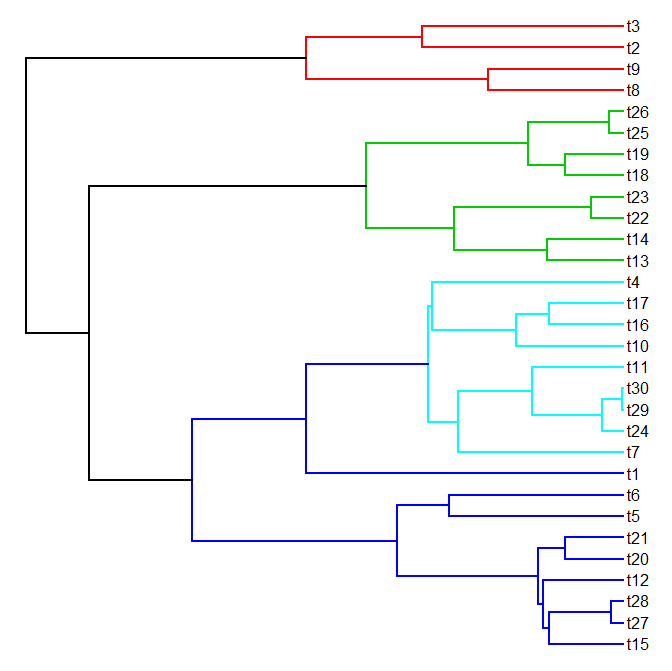
> plotSimmap(tree,pts=FALSE)
no colors provided. using the following legend:
      0        1        2        3        4
"black"    "red" "green3"  "blue"  "cyan"

If we want to use different colors, we can just do:

> cols<-c("black","red","blue","green","purple")
> names(cols)<-0:4
> plotSimmap(tree,cols,pts=FALSE)

If our sole purpose in painting on regimes was to visualize the tree in this way, we could have used the desired colors as regimes. I.e.,

> tree<-paintSubTree(tree,node=31,state="black")
> tree<-paintSubTree(tree,node=57,state="red")
> tree<-paintSubTree(tree,node=50,state="blue")
> tree<-paintSubTree(tree,node=33,state="green")
> tree<-paintSubTree(tree,node=42,state="purple")
> cols<-colnames(tree$mapped.edge)
> names(cols)<-cols
> plotSimmap(tree,cols,pts=FALSE)
to exactly the same effect.

Visualizing different regimes in a phylomorphospace works according to the same principle. Here's a quick demo of that using the same tree:

> X<-fastBM(tree,nsim=2)
> phylomorphospace(tree,X,colors=cols,node.by.map=TRUE, xlab="x",ylab="y")

That's really all there is to it.

Thursday, May 9, 2013

Plotting densityMap using grayscale

Travis Ingram commented that it would be nice to be able to plot density maps using the function densityMap in grayscale. He gave a line of code that could be modified internally to do this; however (as of today!) this is not necessary as we can instead modify our object of class "densityMap" (now returned invisibly by the function) and replot using plot.densityMap. This is what that would look like:

> require(phytools)
Loading required package: phytools
> packageVersion("phytools")
[1] ‘0.2.60’
> # this is just to simulate some data
> tree<-pbtree(n=80,scale=1)
> Q<-matrix(c(-1,1,1,-1),2,2)
> rownames(Q)<-colnames(Q)<-c(0,1)
> tree<-sim.history(tree,Q)
> x<-tree$states
> mtrees<-make.simmap(tree,x,nsim=100)
make.simmap is sampling character histories conditioned on the transition matrix
Q =
        0        1
0 -1.25418  1.25418
1  1.25418 -1.25418
(estimated using likelihood);
and (mean) root node prior probabilities
pi =
  0  1
0.5 0.5
Done.
> # we don't care about this plot
> maps<-densityMap(mtrees,res=500)
sorry - this might take a while; please be patient
> # now let's change our colormap using Travis's code
> maps$cols[]<-grey(seq(1,0,length.out=length(maps$cols)))
> plot(maps,fsize=c(0.6,1),outline=TRUE,lwd=5)

(Click for higher res version.) Cool.

Thanks to Travis for the great suggestion & code.

New version of densityMap

The full title of this post should read New much faster version of densityMap that returns the plotted map invisibly combined with generic plotting method for special mapping object class, or something like that - but that seemed like a tongue twister. densityMap is a function to visualize the posterior sample of maps from a stochastic mapping analysis and is described in an article that I have in press at Methods in Ecology & Evolution.

I just posted a new version of densityMap (code here) that simultaneously addresses a couple of significant issues with this (otherwise pretty cool, in my opinion) function.

Firstly, prior versions of the function are way too slow. The function is still slow - just no longer way too slow. This speed-up was achieved entirely using the trick of removing the class attribute of our "multiPhylo" object which - for some reason that is not entirely clear to me - dramatically speeds up handling of the object both by apply family functions, and even in for loops.

Secondly, what makes densityMap especially annoying to work with - given that it is slow - is that to alter any of the plotting options, you need to re-compute the aggregate mappings. In the new version of densityMap (and new minor phytools build, phytools 0.2-60), densityMap plots the mapped tree as before, but also returns a special object of class "densityMap" invisibly. This can then be plotted using a call of the generic plot (to which I have added the phytools method plot.densityMap).

Here's a demo:

> require(phytools)
Loading required package: phytools
> packageVersion("phytools")
[1] ‘0.2.60’
> # simulate tree & data
> tree<-pbtree(n=70,scale=1)
> Q<-matrix(c(-1,1,1,-1),2,2)
> rownames(Q)<-colnames(Q)<-c(0,1)
> tree<-sim.history(tree,Q)
> x<-tree$states
> # generate stochastic maps
> mtrees<-make.simmap(tree,x,nsim=100)
make.simmap is sampling character histories conditioned on the transition matrix
Q =
          0          1
0 -0.8857354  0.8857354
1  0.8857354 -0.8857354
(estimated using likelihood);
and (mean) root node prior probabilities
pi =
  0  1
0.5 0.5
Done.
> # generate density map
> # this would have been much slower before
> system.time(map<-densityMap(mtrees))
sorry - this might take a while; please be patient
  user  system elapsed
  7.85    0.12    7.97

Now, in earlier versions of densityMap if we wanted to adjust the way this plot looked (say - so that the labels don't overlap!) - we would have to recompute the aggregate mapping (which, remember, took us 8s here - but much longer in earlier versions or for bigger trees). However, here we have created the object maps, which we can then pass to plot.densityMap with our revised plotting options:

> plot(map,lwd=5,fsize=c(0.7,1),legend=0.4)
for example.

Cool.

Wednesday, May 8, 2013

Bug fix & update to phylomorphospace

Yesterday a phytools user identified a bug in the node-coloring of phylomorphospace. I thought that this was likely introduced when I recently did a major rewrite of the function (described here) and this seems to be correct. I have fixed this, and also added a new feature to the function that (for trees with a mapped discrete character) will automatically color nodes using the color of the mapped discrete character. The code of the updated function is here; and I have also posted a new phytools build (phytools 0.2-59).

Here's a demo of the fixed node coloring:

> require(phytools)
Loading required package: phytools
> packageVersion("phytools")
[1] ‘0.2.59’
> # first let's simulate a tree & data
> tree<-pbtree(n=30,scale=1)
> XX<-fastBM(tree,nsim=2)
> plotTree(tree,node.numbers=T)
> # now let's say we want to plot nodes
> # descended from "49" red:
> cols<-rep("black",length(tree$tip.label)+tree$Nnode)
> names(cols)<-1:length(cols)
> cols[getDescendants(tree,49)]<-"red"
> # and everything from "40" blue:
> cols[getDescendants(tree,40)]<-"blue"
> # finally, these can even be nested
> cols[getDescendants(tree,44)]<-"yellow"
> # and plot
> phylomorphospace(tree,XX,xlab="X1",ylab="X2", control=list(col.node=cols))
Cool. (This is basically the demo that I gave in an earlier post.)

Now, when I was doing this I realized that it might be cool to be able to color the nodes - as well as the edges - according to a mapped discrete character. To do this, we need to be able to compute the colors of all internal nodes on the tree from their states. Here is the code that I used to do that:

zz<-c(getStates(tree,type ="tips"), getStates(tree))
names(zz)[1:length(tree$tip.label)]<-
  sapply(names(zz)[1:length(tree$tip.label)],
  function(x,y) which(y==x),y=tree$tip.label)
con$col.node<-setNames(colors[zz],names(zz))
The first line just computes the states at all tip & internal nodes using getStates; the second is just a complicated way of translating tip labels in names(zz) into node numbers, which is what is need by phylomorphospace; finally, line three translates the node states to colors.

Here is a demo:

> # transition matrix
> Q<-matrix(c(-2,2,2,-2),2,2)
> colnames(Q)<-rownames(Q)<-letters[1:2]
> # simulate stochastic history
> tree<-sim.history(tree,Q)
> phylomorphospace(tree,XX,xlab="X1",ylab="X2", colors=setNames(c("blue","red"),letters[1:2]), node.by.map=TRUE)

That's it.

Much faster versions of countSimmap, describe.simmap, and getStates

Yesterday, Klaus Schliep pointed out that a trick to speed up lapply's handling of objects of class "multiPhylo" (i.e., just a simple list of objects of class "phylo") was just to first remove the class attribute "multiPhylo". Why this would have any effect at all is somewhat of a mystery to me. is.list(trees) evaluates TRUE regardless of whether or not the class attribute has been removed, so it doesn't seem that lapply would have to coerce our object to a list in either case. Nonetheless - not only does this work, it works tremendously! I have now included this simple trick in countSimmap, describe.simmap, and getStates, all of which use lapply or sapply if the argument tree is an object of class "multiPhylo".

Here's a demo of just how much of an improvement in speed results from this trick:

> require(phytools)
Loading required package: phytools
> packageVersion("phytools")
[1] ‘0.2.56’
>
> # simulate data
> tree<-pbtree(n=100,scale=1)
> Q<-matrix(c(-1,1,1,-1),2,2)
> colnames(Q)<-rownames(Q)<-letters[1:2]
> tree<-sim.history(tree,Q)
> x<-tree$states
>
> # stochastic mapping
> mtrees<-make.simmap(tree,x,nsim=1000)
make.simmap is sampling character histories conditioned on the transition matrix
Q =
          a          b
a -0.8686634  0.8686634
b  0.8686634 -0.8686634
(estimated using likelihood);
and (mean) root node prior probabilities
pi =
  a  b
0.5 0.5
Done.
>
> # ok, now let's time describe.simmap for
> # various subsets of our mapped trees
> system.time(X100<-describe.simmap(mtrees[1:100], message=FALSE))
  user  system elapsed
  2.69    0.02    2.70
> system.time(X200<-describe.simmap(mtrees[1:200], message=FALSE))
  user  system elapsed
  12.71    0.02  12.75
> system.time(X400<-describe.simmap(mtrees[1:400], message=FALSE))
  user  system elapsed
  74.24    0.64  75.57

Woah. I'm not even going to try the full set of 1,000 trees.

OK, now let's compare to describe.simmap with nothing more than the trick suggested by Klaus (i.e., unclass-ing the "multiPhylo" object for every use of lapply or sapply):

> require(phytools)
Loading required package: phytools
> packageVersion("phytools")
[1] ‘0.2.58’
> system.time(Y100<-describe.simmap(mtrees[1:100], message=FALSE))
  user  system elapsed
  0.45    0.00    0.45
> system.time(Y200<-describe.simmap(mtrees[1:200], message=FALSE))
  user  system elapsed
  0.83    0.00    0.82
> system.time(Y400<-describe.simmap(mtrees[1:400], message=FALSE))
  user  system elapsed
  1.78    0.00    1.78
Holy cow! What a huge improvement. We can even now run it on the full set of 1,000 mapped trees:
> par(cex=0.8) # make our tip labels a little smaller
> system.time(YY<-describe.simmap(mtrees,plot=TRUE))
1000 trees with a mapped discrete character with states:
a, b

trees have 29.633 changes between states on average

changes are of the following types:
        a,b    b,a
x->y 10.692 18.941

mean total time spent in each state is:
              a          b    total
raw  12.9314025 18.3673136 31.29872
prop  0.4131608  0.5868392  1.00000

  user  system elapsed
  4.65    0.06    4.71

Wow.

Tuesday, May 7, 2013

Faster version of getStates, but why is it faster...?

I was tinkering with the function describe.simmap to try and speed it up, when I discovered that the very simple function getStates, which does nothing more than get the states on a mapped tree in memory for the nodes or tips, had run-time using lapply to iterate over the trees in an object of class "multiPhylo", that seems to rise non-linearly with the number of trees.

> ## simulate tree & data
> tree<-pbtree(n=200,scale=1)
> Q<-matrix(c(-1,1,1,-1),2,2)
> colnames(Q)<-rownames(Q)<-letters[1:2]
> trees<-sim.history(tree,Q,nsim=200)
> # now lets get the states for all trees at all nodes
> # using sapply
> system.time(XX1<-getStates(trees[[1]]))
  user  system elapsed
  0.02    0.00    0.02
> system.time(XX10<-sapply(trees[1:10],getStates))
  user  system elapsed
  0.05    0.00    0.04
> system.time(XX50<-sapply(trees[1:50],getStates))
  user  system elapsed
  0.28    0.00    0.29
> system.time(XX100<-sapply(trees[1:100],getStates))
  user  system elapsed
  1.16    0.00    1.16
> system.time(XX200<-sapply(trees,getStates))
  user  system elapsed
    6.6    0.0    6.6

Hmmm. What's going on here?

What I discovered (somehow - I'm not sure why I tried this) is that if I first split my list of 200 trees into, say, 20 lists of 10 trees; and then I ran sapply(...,getStates) on each of these lists; then recombined the results using cbind, this is much faster. So, for instance:

> g<-function(trees){
 ff<-as.factor(ceiling(1:length(trees)/10))
 aa<-lapply(split(trees,ff),function(x)   sapply(x,getStates))
 y<-if(length(trees)>10) aa[[1]] else aa
 for(i in 2:length(aa)) y<-cbind(y,aa[[i]])
 y
}
> # now run it
> system.time(YY200<-g(trees))
  user  system elapsed
  0.97    0.00    0.97
> # check all equal
> dim(YY200)
[1] 199 200
> dim(XX200)
[1] 199 200
> all(XX200==YY200)
[1] TRUE

Seriously - what's going on here? (I have some ideas - but I'm not sure. Feedback welcome.)

Here's a new version of getStates with this hack implemented internally:

# function to get node states from simmap style trees
# written by Liam J. Revell 2013
getStates<-function(tree,type=c("nodes","tips")){
  type<-type[1]
  if(class(tree)=="multiPhylo"){
    ff<-as.factor(ceiling(1:length(tree)/10))
    aa<-lapply(split(tree,ff),function(x)
     sapply(x,getStates))
    y<-if(length(tree)>10) aa[[1]] else aa
    for(i in 2:length(aa)) y<-cbind(y,aa[[i]])
  } else if(class(tree)=="phylo"){
    if(type=="nodes"){
      y<-setNames(sapply(tree$maps,function(x)
       names(x)[1]),tree$edge[,1])
      y<-y[as.character(length(tree$tip)+1:tree$Nnode)]
    } else if(type=="tips"){
      y<-setNames(sapply(tree$maps,function(x)
       names(x)[length(x)]),tree$edge[,2])
      y<-setNames(y[as.character(1:length(tree$tip))],
       tree$tip)
    }
  } else stop("tree should be an object of class 'phylo' or 'multiPhylo'")
  return(y)
}

Saturday, May 4, 2013

Huge speed-up for rerootingMethod & estDiversity

A couple of months ago I posted an extremely simple function - basically a wrapper for the 'ape' function ace - to do marginal ancestral state reconstruction using the re-rooting method of Yang.

Well - this function is quite slow. This is partly because the tree has to be re-rooted at every internal node; but mostly this is slow for a totally unnecessary reason, and that is that by wrapping around ace (or, rather, a very lightly modified version of ace used internally by phytools), at each re-rooting the function also re-estimates the transition matrix, Q. Obviously - since only symmetric transition matrices are permitted by this method - this is totally unnecessary.

This is now fixed in the latest minor phytools build (phytools 0.2-56) and the result is an enormous speed-up in computation time. So, for instance:

> require(phytools)
Loading required package: phytools
> packageVersion("phytools")
[1] ‘0.2.55’
>
> # simulate
> tree<-pbtree(n=100,scale=1)
> Q<-matrix(c(-2,1,1,1,-2,1,1,1,-2),3,3)
> rownames(Q)<-colnames(Q)<-letters[1:3]
> x<-sim.history(tree,Q)$states
>
> # ok, now estimate using the old version
> system.time(XX<-rerootingMethod(tree,x))
  user  system elapsed
  28.34    0.00  28.42
> # unload phytools and install the new version
> detach("package:phytools",unload=TRUE)
> install.packages("phytools_0.2-56.tar.gz",type="source", repos=NULL)
* installing *source* package 'phytools' ...
** R
...
* DONE (phytools)
> require(phytools)
Loading required package: phytools
> packageVersion("phytools")
[1] ‘0.2.56’
>
> # ok, now repeate the analysis using the new version
> system.time(YY<-rerootingMethod(tree,x))
  user  system elapsed
  3.36    0.01    3.38
> plot(XX$marginal.anc,YY$marginal.anc,xlab="marginal ASRs old version",ylab="marginal ASRs new version")

Cool.

The same speed-up can also be applied to estDiversity - which estimates historical lineage diversity at all the nodes of the tree based on the approach of Mahler et al. (2010) (e.g., 1, 2). So, for instance:

> require(phytools)
Loading required package: phytools
> packageVersion("phytools")
[1] ‘0.2.55’
>
> system.time(d.old<-estDiversity(tree,x))
Please wait. . . . Warning - this may take a while!
Completed 10 nodes
Completed 20 nodes
Completed 30 nodes
Completed 40 nodes
  user  system elapsed
 228.64    0.14  236.39
>
> detach("package:phytools",unload=TRUE)
> install.packages("phytools_0.2-56.tar.gz",type="source", repos=NULL)
...
* DONE (phytools)
> require(phytools)
Loading required package: phytools
> packageVersion("phytools")
[1] ‘0.2.56’
>
> system.time(d.new<-estDiversity(tree,x))
Please wait. . . . Warning - this may take a while!
Completed 10 nodes
Completed 20 nodes
Completed 30 nodes
Completed 40 nodes
  user  system elapsed
  26.02    0.04  26.41
> plot(d.old,d.new,xlab="estimated historical diversity (old)",ylab="estimated historical diversity (new)")

Wow. That's an enormous difference. Cool.

Thursday, May 2, 2013

Bug fix in fastAnc

A couple of days ago a phytools user reported a bug in geomorph (which reverse depends on phytools) that seemed to be due to a problem with fastAnc, which is used internally.

Well, I finally got around to looking into it. It turns out that there was a bug in fastAnc, but I'd overlooked it for good reason - it only occurs under the somewhat idiosyncratic circumstances of when is.binary.tree(tree)=FALSE and the user-specified option vars=FALSE. This is because fastAnc works by re-rooting the tree at all internal nodes of a binary tree and computing the PIC ancestral state & variance. If the input tree is not binary, then it uses multi2di, but then has to back-translate to the original tree which it does using phytools matchNodes.

The problem arose because:

if(!is.binary.tree(tree)){
  ancNames<-matchNodes(tree,btree)
  anc<-anc[as.character(ancNames[,2])]
  names(anc)<-ancNames[,1]
  if(vars) v[as.character(ancNames[,2])]
  names(v)<-ancNames[,1]
}
should have been:
if(!is.binary.tree(tree)){
  ancNames<-matchNodes(tree,btree)
  anc<-anc[as.character(ancNames[,2])]
  names(anc)<-ancNames[,1]
  if(vars||CI){
    v[as.character(ancNames[,2])]
    names(v)<-ancNames[,1]
  }
}
in the code that is executed to back-translate nodes betweeen trees. Basically, if is.binary.tree(tree)=FALSE and vars=FALSE (but under no other circumstances), fastAnc will try to assign names to a vector of zero length. Oops.

The fixed source code for this very simple function is here, but I also posted a new phytools build (phytools 0.2-55).