I just posted a new version of make.simmap that samples stochastic histories not only conditioned on the most likely value of Q, but that can also use a fixed value of Q, or can sample Q from its posterior probability distribution conditioned on the substitution model. Pretty cool!
The motivation underlying this is that prior versions of make.simmap sampled stochastic histories by fixing Q. This is empirical Bayesian because we are fixing one level of the model - in this case, the transition matrix - at its most likely value given the data, rather than sampling from the posterior distribution. This should be unbiased - but it will cause the variance on estimated parameters to be too low. We can see this in the simulation I posted recently - although the effect is small when the tree & tip data contain lots of information about the evolutionary transition rates. By fixing Q we circumvent the (perhaps) challenging tasks of specifying prior densities.
Well, this empirical Bayes method remains available as an option in make.simmap (in fact, as the default - because I think it makes sense for most users) - but now users can also sample Q, rather than merely assuming a fixed value. The way this works is as follows:
1. For each tree, we obtain nsim samples from the posterior distribution by nsim × samplefreq generations of MCMC (after burnin). We also keep the conditional likelihoods from the pruning algorithm from each value of Q in this step.
2. For each value of Q & set of conditional likelihoods, we simulate a set of node states and stochastic map up the tree.
make.simmap uses a γ prior probability distribution for the rates with α & β that can be specified by the user. By default, α = β = 1.0, but this will probably not be a good prior density for your dataset.
make.simmap also offers the option of allowing the data to inform the prior distribution. This is accomplished using make.simmap(...,prior= list(use.empirical=TRUE)). In this case, only β from the specified γ distribution will be used - and α will be set at α = β × ML(Q).
Let's experiment with the function:
[1] ‘0.2.53’
> require(phytools)
Loading required package: phytools
> # simulate data & tree > Q<-matrix(c(-1,1,1,-1),2,2)
> rownames(Q)<-colnames(Q)<-letters[1:2]
> tree<-pbtree(n=100,scale=1)
> tree<-sim.history(tree,Q)
> x<-tree$states
> # describe.simmap on true history
> AA<-describe.simmap(tree,message=FALSE)
> # perform stochastic mappings using the empirical
> # priors method
> mtrees<-make.simmap(tree,tree$states,nsim=100, model="ER",Q="mcmc",prior=list(beta=3,use.empirical=TRUE))
Running MCMC burn-in. Please wait....
Running 10000 generations of MCMC, sampling every 100 generations. Please wait....
make.simmap is simulating with a sample of Q from the posterior distribution
Mean Q from the posterior is
Q =
a b
a -1.009082 1.009082
b 1.009082 -1.009082
and (mean) root node prior probabilities
pi =
[1] 0.5 0.5
Done.
> # describe.simmap on stochastic maps
> XX<-describe.simmap(mtrees,message=FALSE)
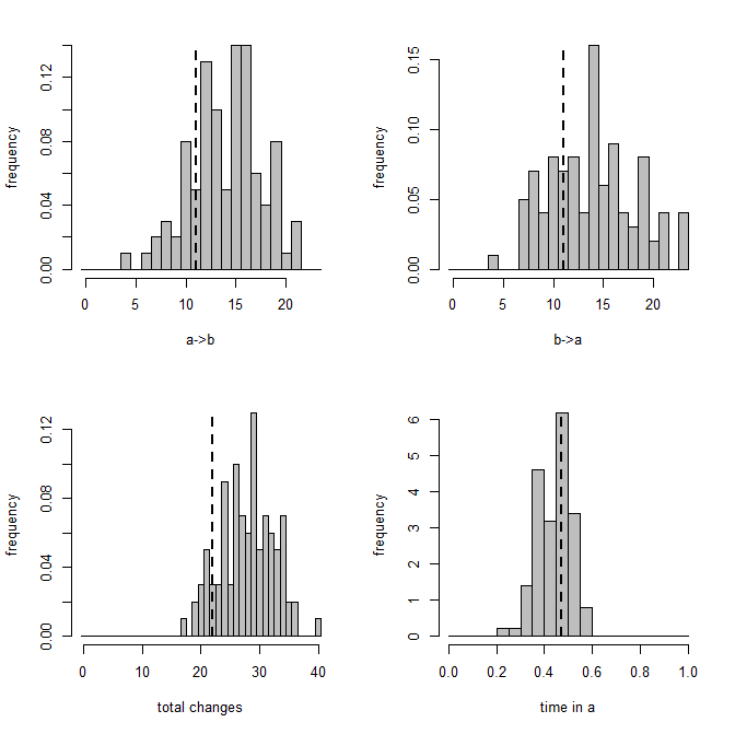
Here's a summary of the results:

Now let's compare to the empirical Bayes method in which we fix Q at its most likely value:
make.simmap is sampling character histories conditioned on the transition matrix
Q =
a b
a -0.9704866 0.9704866
b 0.9704866 -0.9704866
(estimated using likelihood);
and (mean) root node prior probabilities
pi =
a b
0.5 0.5
Done.
> # describe.simmap on stochastic maps
> YY<-describe.simmap(mtrees,message=FALSE)
Some results:
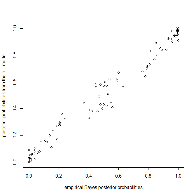
Again, we're seeing more or less what we'd expect - specifically, more uncertainty in the posterior probabilities from the full model in nodes that have posterior probabilities near zero or one in the empirical Bayesian method.
Cool.
This is just a test version - who knows how many bugs will be found before I'm done; however source code is available here, or (if you'd preferred) it is in a new beta build of phytools (phytools 0.2-53) on my website.
Hi Liam, first congrats on the new paper on "Methods". }
ReplyDeleteI wonder how can I alter the size of the "pie" in describe.simmap to fit a big topology.
I can alter the size or scale of the whole drawing in RStudio but it would be wonderful to alter the size of the node-pies first. Is there a similar way to handle it like plotSimmap?
Same question for altering the color ? Would it be via a similar way plotSimmap does it ~ "leg<-c("blue","red")" ?
Try this (tree is your phylogeny, mtrees is your set of stochastic mapped trees):
DeleteXX<-describe.simmap(mtrees)
hh<-max(nodeHeights(tree))
plot(tree,no.margin=TRUE,label.offset=0.02*hh)
nodelabels(pie=XX$ace,piecolors=c("blue","red"),
cex=0.5)
tiplabels(pie=to.matrix(y,seq=colnames(XX$ace)),
piecolors=c("blue","red"),cex=0.5)
You can adjust cex, label.offset, & piecolors as desired.
Let me know if this works. - Liam
This comment has been removed by the author.
ReplyDeleteSorry for the double post, also in the second line I got
ReplyDeleteError in BOTHlabels(text, tip, XX, YY, adj, frame, pch, thermo, pie, piecol, :
could not find function "to.matrix"
Which matrix is being referred?
to.matrix is in the NAMESPACE of phytools now - but it may not have been in earlier version. You can use this:
Deleteto.matrix<-function(x,seq)
sapply(seq,function(x,y) 1*(x==y),y=x)
Sorry this was the previous post, now fixeds since I couldn't edit it.
ReplyDeleteWorked wonderfully for the size, now trying to handle the colors for 3 traits I obtained the third one in green anyway.
I tried:
nodelabels(pie=XX$ace,piecolors=c("blue","red", "orange"),
cex=0.2)
tiplabels(pie=to.matrix (y, seq=colnames(XX$ace)),
piecolors=c("blue","red", "orange"),cex=0.5)
Should I define something else?
Probably should be "piecol" not "piecolors" - that might be your problem. Sorry about that.
DeleteSee more about this here.
Sorry, my mistake. It worked fine.
ReplyDeleteGreat post at the link!
Thanks
Hi Liam,
ReplyDeletereally great stuff. Being able to undertake posterior mapping in R is great. I thought that in response to your comment about priors "but this will probably not be a good prior density for your dataset" readers would be interested in the following article where we explore the effects of the gamma prior on the results (and potential provide a solution).
Maybe you could provide a link within the above text.
Best regards
Thomas
http://www.plosone.org/article/info%3Adoi%2F10.1371%2Fjournal.pone.0010473#pone-0010473-g006
Hi Liam
ReplyDeleteHave you published about this?
Hi,
ReplyDeleteI have a question regarding gamma prior. I'm not sure I understand it correctly. If I use default prior the mean and variance of gamma distribution is equal 1 so the shape of distribution is more similar to exponential function. The problem is what to do to change it to be more similar to log-normal. Should I just take larger value of beta like 3 or 4?
Best
Marcin
Hi Marcin. You could instead increase alpha. If you set one, but not the other, the value of the second will be set automatically to maintain a constant mean of the distribution at the empirical (ML) value of the transition rate, q. That way changing only alpha or beta (but not both) changes only the shape of the gamma distribution, but not its mean.
DeleteYou might also try:
plot(dgamma(x,alpha,beta))
(in which x is a vector in the horizontal dimension) to see how different distributions look.
Hi Liam,
ReplyDeleteGreat function!
I was wondering if I could fix some ancestral states in this function.
Is that possible?
Thanks