I wanted to repeat & elaborate some performance testing that I conducted earlier in the month. This is partly motivated by the fact that I introduced and then fixed a bug in the function since conducting this test; and partly this is driven by some efforts to figure out why the stand-alone program SIMMAP can give deceptively misleading results when the default priors are used (probably because the default priors should not be used - more on this later).
My simulation test was as follows:
1. I simulated a stochastic phylogeny (using pbtree) and character history for a binary trait with states a and b (using sim.history) conditioned on a fixed, symmetric transition matrix Q. For these analyses, I simulated a tree with 100 taxa of total length 1.0 with backward & forward rate of 1.0.
2. I counted the true number of transitions from a to b & b to a; the true total number of changes; and the true fraction of time spent in state a (for any tree, the time spent in b will just be 1.0 minus this).
3. I generated 200 stochastic character maps using make.simmap. For more information about stochastic mapping or make.simmap search my blog & look at appropriate references.
4. From the stochastic maps, I computed the mean number of transitions of each type; the mean total number of changes; and the mean time spent in state a. I evaluated whether the 95% CI for each of these variables included the true values from 1.
5. I repeated 1. through 4. 200 times.
First, we can ask how often the 95% CI includes the generating values. Ideally, this should be 0.95 of the time:
a,b b,a N time.a
0.905 0.895 0.790 0.950
Now let's attach some visuals to parameter estimation. Figure 1 shows scatterplots of the relationship between the true and estimated (averaged across 200 stochastic maps) values of each of the four metrics described above:
Figure 1:
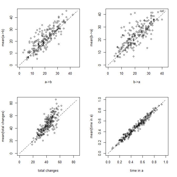
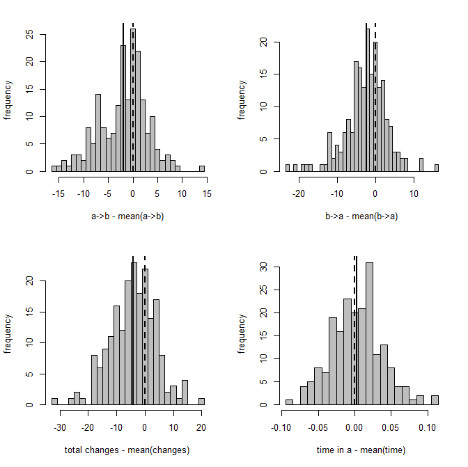
Figure 2 is a clearer picture of bias. It gives the distribution of Y - Ŷ, where Ŷ is just the mean from the stochastic maps for a given tree & dataset. The vertical dashed line gives the expectation (zero) if our method is unbiased; whereas the vertical solid line is the mean of our sample.
Figure 2:
That's it. I'm not posting the code - because there's a whole bunch of it; however if you want it, please just let me know.
Hi Liam! This is all very exciting, and I can't wait to hear more about it as you compare the two procedures, as it is something I've been dealing with in a way for my data.
ReplyDeleteOne thing I noticed using this approach for my data is that SIMMAP tends to generate maps that have considerably less transitions, especially for rare tip states. When I use make.simmap for the same data, I tend to get far more transitions (for one dataset, I remember getting like 10 times more frequent shifts for one transition type, even when using a non-symmetrical transition matrix), and many more of those "within-branch transition sandwiches" (you know? when in a single branch, the map will shift from state 0 to state 1, then back to state 0).
Since these are all in the case of empirical data, I don't know the true transition probabilities and thus it becomes hard to evaluate which procedure is returning something closer to the underlying real model. I tend to find that SIMMAP produces results that are more intuitive and with fewer of the above mentioned (and ridiculously named) "sandwiches". In any case, I thought I would share my case; I wonder if this is something you've ran into before and what are your thoughts.
Cheers!
Hi Rafael.
DeleteThis exactly the same result that has been motivating some of these analyses!
I'm beginning to figure out that this is due to SIMMAP users putting a strong prior on the rate in SIMMAP to be too low. The consequence is that sampled histories have too few changes.
There are other consequences as well - for instance, posterior probabilities at nodes >0.5 will be pushed up and <0.5 will be pushed down. This gives us incorrect (over)confidence in nodal reconstructions if they are taken from the sample of maps.
An easy "back of the envelope" cross-check of whether SIMMAP is giving you a number of changes that is consistent with your empirical rates can be performed as follows: 1. fit the "ER" model using ace or fitDiscrete; (if the fit of the "ER" model is not much worse than other models) 2. compute sum(tree$edge.length)*(-qii) in which qii is any element on the diagonal of Q (equal to -m*qij for m states under the model "ER") - this gives you the expected number of changes under the model, which you can then compare to the number from SIMMAP.
make.simmap avoids this issue by fixing one level of the model - the transition matrix, Q - at it's most likely value, rather than sampling over uncertainty in Q. The consequence is that the number of changes is estimated unbiasedly - but that the CI from the posterior sample is slightly too small. This is better than using a strong, "misleading" prior on Q (in the loose sense that it is inconsistent with the empirical rate - in Bayesian analyses we can choose to put a high weight on our prior belief, but I don't think that most SIMMAP users intend to do this), which will cause SIMMAP to be biased with high confidence.
My empirical validation of this conclusion comes from taking a dataset of trees from SIMMAP shared with me by a colleague and comparing them to mappings from make.simmap with various (downward relative to the empirical rate, in this case) constraints imposed on Q. What I find is that I can replicate the results of SIMMAP by constraining Q to be (in this case) 1/4 of its empirical most likely value.
We will also find as we put a stronger & stronger downward prior on Q our reconstructed histories will converge to the parsimony reconstructions. This means that if we have a large effect of the prior distribution on Q being too low, our reconstructions will seem very sensible - because they are parsimonious! Of course, we all know that parsimony will give us a biased picture of the true number of changes on the tree because "hidden" changes are not represented in our sample. Again, this is super easy to show using make.simmap by constraining Q during the "empirical" phase of estimation. If you do this for lower & lower maximum values of Q, then eventually the mean number of changes across stochastic maps will go to the parsimony score for the character & tree. In the limiting case, all the trees will have a number of changes equal to the parsimony score. Although there will still be uncertainty in the states at some nodes, this is due to their being multiple equally parsimonious reconstructions!
Now, I do not think that this is a problem with SIMMAP - just with our natural tendency to use the default settings. This is combined (dangerously) with the fact that if the bias created by the prior on Q is for Q to be much lower than its empirical value, this will have the effect of making our reconstructions look nice & parsimonious.
Thanks for the comment as it reinforces my impression that this is an important issue.
- Liam
Also see this post: blog.phytools.org/2013/04/stochastic-mapping-with-bad-informative.html. - Liam
DeleteHi Liam,
Deletemany thanks for the very thorough response. Yes, this makes a lot of sense - how, by converging on the parsimony result, we get an intuitive (but wrong) reconstruction! This is quite unexpected to me, not knowing many of the "under the hood" details, but makes a lot of sense - and is important to know! Even in the SIMMAP documentation, I can remember reading something about the default priors not being appropriate for most cases, but I'm sure that many people probably had the same reaction that I had - "well, looks fine to me, my case is probably not like most cases!".
I'm going to play around with this and my data to see what comes out (once I finish this last week of teaching!). One thing that bothers me a bit is still the "regime sandwiches", because in most cases they seem to me to be pretty biologically meaningless - for example, not unusual for a red branch to pop in and out in a clade that is pretty much entirely black. Except maybe in a threshold model, where it is reasonable that some clades will fluctuate near the threshold. But in a purely mendelian type of binary/qualitative trait it becomes hard to interpret these biologically - which I guess is not really relevant for this method, where these sandwiches are simply representing uncertainty in the reconstruction of that branch once you consider multiple reconstructions, am I right?
Thanks again for clarifying this - and also for bringing this up to our attention!
Hi Rafael.
DeleteNo, the sandwiches are valid realizations of the evolutionary process given the model. If the data for the tips suggest that the rate of evolution for the discrete character is high, then sometimes (under a high rate) the state for the character will flip back & forth along an individual branch. The higher the rate that is implied by the data, the more sandwiches you will see.
If you think this is implausible for your data, you are essentially being a Bayesian & saying: "even though the data would suggest that the character changes frequently (i.e., at a high rate), my prior belief is that changes in the character are very difficult and thus should only occur infrequently. I'd thus prefer a reconstructed history that minimally conflicts with this prior belief - e.g., the parsimony reconstruction."
Note, of course, that as I've emphasized in the past the stochastic maps can only be considered in aggregate. Any individual sandwich is highly improbable - however (if the rate is sufficiently high) some number of hidden changes ("sandwiches") are virtually guaranteed under the model.
Great discussion. Thanks Rafael.
- Liam
Here's a test comment.
ReplyDeleteSee:
http://productforums.google.com/d/topic/blogger/oXxuvPSFnpo/discussion
Thanks Admin for sharing such a useful post, I hope it’s useful to many individuals for whose looking this precious information to developing their skill.
ReplyDeleteRegards,
Best software testing training institute in chennai|Software testing courses in chennai|testing training chennai