Showing posterior probabilities from describe.simmap at the nodes of a plotted tree

A user comment asks the following:

"I wonder how can I alter the size of the "pie" in describe.simmap.... Same question for altering the color...."

Well, there is no way at present to change the color or pie-size in describe.simmap(...,plot=TRUE); however, describe.simmap, it is easy to recreate the posterior probability plot of describe.simmap using the function output - while customizing its attributes.

Here's a quick demo:

> # check package version
> packageVersion("phytools")
[1] ‘0.2.54’
>
> # first simulate some data to use in the demo
> Q<-matrix(c(-2,1,1,1,-2,1,1,1,-2),3,3)
> rownames(Q)<-colnames(Q)<-letters[1:3]
> tree<-sim.history(pbtree(n=50,scale=1),Q)
> x<-tree$states
>
> # now the demo
> mtrees<-make.simmap(tree,x,model="ER",nsim=100)
make.simmap is sampling character histories conditioned on the transition matrix
Q =
          a        b        c
a -2.041867  1.020934  1.020934
b  1.020934 -2.041867  1.020934
c  1.020934  1.020934 -2.041867
(estimated using likelihood);
and (mean) root node prior probabilities
pi =
        a        b        c
0.3333333 0.3333333 0.3333333
Done.
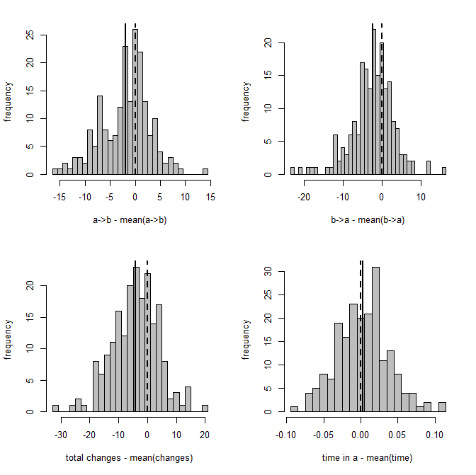
> XX<-describe.simmap(mtrees,plot=FALSE)
100 trees with a mapped discrete character with states:
a, b, c

trees have 23.93 changes between states on average

changes are of the following types:
      a,b  a,c  b,a  b,c  c,a  c,b
x->y 2.11 2.91 4.62 5.77 4.94 3.58

mean total time spent in each state is:
            a        b        c    total
raw  2.2816521 4.1930936 4.2593925 10.73414
prop 0.2125603 0.3906316 0.3968081  1.00000

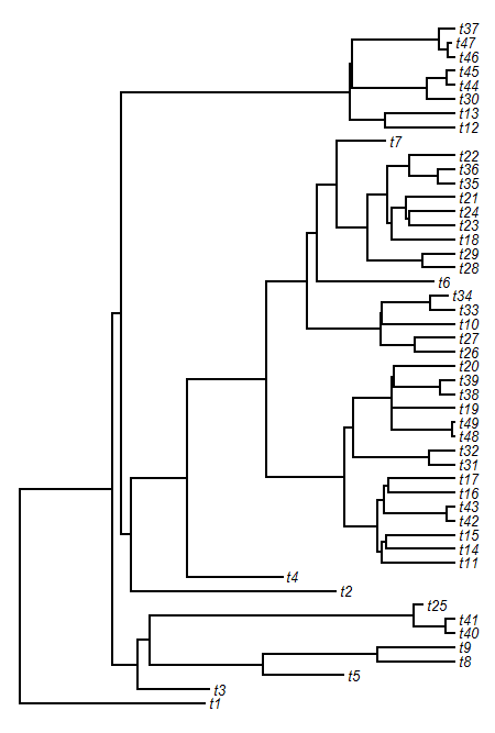
> hh<-max(nodeHeights(tree))*0.02 # for label offset
> plot(tree,no.margin=TRUE,label.offset=hh,edge.width=2)
> nodelabels(pie=XX$ace,piecol=c("blue","red","green"), cex=0.5)
> tiplabels(pie=to.matrix(x,colnames(XX$ace)), piecol=c("blue","red","green"),cex=0.5)

Obviously, to adjust the pie-sizes & colors we just change the values of cex & piecol.

That's it.

New article describing new graphical methods: densityMap, contMap, and fancyTree(...,type="phenogram95")

My new article describing three new graphical methods for plotting comparative data on trees, implemented in the phytools functions densityMap (1, 2, 3, 4), contMap (1, 2, 3), and fancyTree(..., type="phenogram95") just came out "Accepted" (i.e., manuscript pages, not type-set or proofed) in Methods in Ecology & Evolution. The article is entitled Two new graphical methods for mapping trait evolution on phylogenies, which might seem like a bit of a misnomer (or perhaps a tribute to this article) given my description, above, but I think it makes sense.

The figure at right is from the paper (click for a larger version with tip labels). Thanks to Dave Collar for helpfully providing the published data & tree.

2x faster version of make.simmap for Q="mcmc"

In a previous post I promised that I could speed up make.simmap(..., Q="mcmc"), i.e., the full Bayesian MCMC make.simmap method. (Matt Pennell said he didn't care, which is very generous of him.)

There was one really low-hanging fruit which is that during Bayesian MCMC sampling of the transition matrix, Q, make.simmap was unnecessarily computing the likelihood twice for each iteration of the MCMC. This is because make.simmap uses modified code from ape's ace function internally to perform Felsenstein's pruning algorithm in computing the likelihood of Q as well as well as the conditional scaled likelihoods at each node. Normally, ace returns the likelihood & the scaled conditional likelihoods of the subtrees at each internal node by first maximizing the likelihood using the optimizer nlminb, and the computing the conditional likelihoods given MLE(Q). I modified the code to take a fixed value of Q, however it still returned both the overall log-likelihood & the conditional likelihoods via two rounds of the pruning algorithm. For the vast majority of generations in our MCMC we don't care about the conditional scaled likelihoods (because we're not sampling that generation) so we should only compute the overall log-likelihood which we need to compute the posterior odds ratio and make a decision about whether to retain the updated parameter values or not. Whenever we want to sample a particular value for Q (i.e., every samplefreq generations), we can compute the conditional likelihoods for all the nodes - since we'll need these later.

This improvement has a pretty dramatic effect on computation time - pretty much halving it as you might expect. Here's a demo using my not-too-fast i5 desktop:

> # simulate tree & data
> Q<-matrix(c(-1,1,1,-1),2,2)
> colnames(Q)<-rownames(Q)<-LETTERS[1:2]
> tree<-sim.history(pbtree(n=100,scale=1),Q)
> x<-tree$states
> # number of changes, etc., on the true tree
> describe.simmap(tree)
1 tree with a mapped discrete character with states:
 A, B

tree has 21 changes between states

changes are of the following types:
  A  B
A  0 11
B 10  0

mean total time spent in each state is:
              A          B    total
raw  11.5075650 10.5967548 22.10432
prop  0.5206025  0.4793975  1.00000

> # OK, now let's run make.simmap & time it
> system.time(mtrees.old<-make.simmap(tree,x,Q="mcmc", nsim=200,prior=list(beta=2,use.empirical=TRUE)))
Running MCMC burn-in. Please wait....
Running 20000 generations of MCMC, sampling every 100 generations. Please wait....
make.simmap is simulating with a sample of Q from the posterior distribution
Mean Q from the posterior is
Q =
          A        B
A -1.205146  1.205146
B  1.205146 -1.205146
and (mean) root node prior probabilities
pi =
[1] 0.5 0.5
Done.
  user  system elapsed
398.44    0.23  401.99
> # pretty slow!!
> describe.simmap(mtrees.old)
200 trees with a mapped discrete character with states:
 A, B

trees have 29.93 changes between states on average

changes are of the following types:
        A,B    B,A
x->y 15.055 14.875

mean total time spent in each state is:
              A          B    total
raw  11.3629822 10.7413376 22.10432
prop  0.5140616  0.4859384  1.00000

OK - now let's compare to the updated version:

> source("make.simmap.R")
> system.time(mtrees.new<-make.simmap(tree,x,Q="mcmc", nsim=200,prior=list(beta=2,use.empirical=TRUE)))
Running MCMC burn-in. Please wait....
Running 20000 generations of MCMC, sampling every 100 generations. Please wait....
make.simmap is simulating with a sample of Q from the posterior distribution
Mean Q from the posterior is
Q =
          A        B
A -1.227405  1.227405
B  1.227405 -1.227405
and (mean) root node prior probabilities
pi =
[1] 0.5 0.5
Done.
  user  system elapsed
214.87    0.03  216.36
> # still slow, but better
> describe.simmap(mtrees.new)
200 trees with a mapped discrete character with states:
 A, B

trees have 29.975 changes between states on average

changes are of the following types:
        A,B  B,A
x->y 14.585 15.39

mean total time spent in each state is:
              A          B    total
raw  11.1900994 10.9142203 22.10432
prop  0.5062404  0.4937596  1.00000

The code for this version is here, but I have also posted a new phytools build (phytools 0.2-54). Check it out & please report any issues or bugs.

Stochastic mapping with a bad informative prior results in parsimony reconstruction

The title to this post pretty much says it all. As alluded to in the discussion thread of an earlier post, if you use an informative prior probability distribution in which the mean is too low - then the result can (especially in the limiting case as the mean goes to zero) become the parsimony reconstruction. That is, as our prior probability distribution forces our posterior distribution of Q to be closer & closer to zero, all reconstructions converge to the one or multiple most parsimonious reconstructions.

Here's a quick demonstration of what I mean. Just to make the point clear, I have used a very exaggerated bad prior probability density - the γ with α = 2 & β = 200 - which basically says we have a high degree of confidence that the rate of evolution is very low (with mean α/β = 0.01).

> library(phytools)
Attaching package: ‘phytools’

> # first create a mapped history
> Q<-matrix(c(-2,2,2,-2),2,2)
> colnames(Q)<-rownames(Q)<-LETTERS[1:2]
> tree<-sim.history(pbtree(n=100,scale=1),Q,anc="A")
> describe.simmap(tree)
1 tree with a mapped discrete character with states:
A, B

tree has 54 changes between states

changes are of the following types:
   A  B
A  0 18
B 36  0

mean total time spent in each state is:
             A         B    total
raw  12.897944 15.049629 27.94757
prop  0.461505  0.538495  1.00000

> x<-tree$states
> # now let's perform stochastic mapping with a
> # reasonable prior
> emp.prior<-make.simmap(tree,x,nsim=100,Q="mcmc", prior=list(beta=2,use.empirical=TRUE))
Running MCMC burn-in. Please wait....
Running 10000 generations of MCMC, sampling every 100 generations. Please wait....
make.simmap is simulating with a sample of Q from the posterior distribution
Mean Q from the posterior is
Q =
          A        B
A -1.943666  1.943666
B  1.943666 -1.943666
and (mean) root node prior probabilities
pi =
[1] 0.5 0.5
Done.

> # now a prior that is way too low!
> low.prior<-make.simmap(tree,x,nsim=100,Q="mcmc", prior=list(alpha=2,beta=200))
Running MCMC burn-in. Please wait....
Running 10000 generations of MCMC, sampling every 100 generations. Please wait....
make.simmap is simulating with a sample of Q from the posterior distribution
Mean Q from the posterior is
Q =
          A          B
A -0.1103515  0.1103515
B  0.1103515 -0.1103515
and (mean) root node prior probabilities
pi =
[1] 0.5 0.5
Done.

> # plot all three for comparison to the true tree
> layout(matrix(c(1,2,3),1,3))
> plotSimmap(tree,pts=F,lwd=2,ftype="off")
no colors provided. using the following legend:
      A      B
"black"  "red"
> plotSimmap(emp.prior[[1]],pts=F,lwd=2,ftype="off")
...
> plotSimmap(low.prior[[1]],pts=F,lwd=2,ftype="off")
...

What's dangerous about the reconstructions shown above is that (without the known true history, as in this case) it may be the rightmost reconstruction - the one obtained with the faulty prior - that looks most reasonable!

OK - let's do a little more analysis to further the point:

> describe.simmap(emp.prior)
100 trees with a mapped discrete character with states:
A, B

trees have 60.09 changes between states on average

changes are of the following types:
      A,B  B,A
x->y 29.52 30.57

mean total time spent in each state is:
              A          B    total
raw  15.7298487 12.2177248 27.94757
prop  0.5628341  0.4371659  1.00000

> describe.simmap(low.prior)
100 trees with a mapped discrete character with states:
A, B

trees have 22.97 changes between states on average

changes are of the following types:
      A,B  B,A
x->y 14.44 8.53

mean total time spent in each state is:
              A          B    total
raw  17.7439790 10.2035945 27.94757
prop  0.6349023  0.3650977  1.00000

> # get parsimony score
> library(phangorn)
> X<-phyDat(as.matrix(x),type="USER",levels=LETTERS[1:2])
> parsimony(tree,X)
[1] 22

Of course, we can push it even further & virtually guarantee that our stochastic maps have the MP number of changes, e.g.:

> really.low.prior<-make.simmap(tree,x,nsim=20,Q="mcmc", prior=list(alpha=1,beta=1e4))
Running MCMC burn-in. Please wait....
Running 2000 generations of MCMC, sampling every 100 generations. Please wait....
make.simmap is simulating with a sample of Q from the posterior distribution
Mean Q from the posterior is
Q =
            A            B
A -0.002198051  0.002198051
B  0.002198051 -0.002198051
and (mean) root node prior probabilities
pi =
[1] 0.5 0.5
Done.
> describe.simmap(really.low.prior)
20 trees with a mapped discrete character with states:
A, B

trees have 22.05 changes between states on average

changes are of the following types:
      A,B B,A
x->y 13.65 8.4

mean total time spent in each state is:
              A          B    total
raw  17.4916200 10.4559534 27.94757
prop  0.6258726  0.3741274  1.00000

Well, you get the idea.

Method comparison in make.simmap

A couple of days ago I introduced a new version of make.simmap that uses Bayesian MCMC to sample the transition matrix, Q, from its posterior probability distribution rather than fixing it at the MLE (as in previous versions of the function). The idea is that by fixing Q we are ignoring variation in the reconstructed evolutionary process that is due to uncertainty in the transition matrix.

I thought that, as a first pass, it might be neat to compare these two approaches: one in which we fix Q at its most likely value; and the other in which Q is sampled from its posterior probability distribution. My expectation is relatively straightforward - variance on estimated variables should go up (hopefully towards their true variance), and the probability that the generating parameter values should be on their corresponding (1-α)% CIs (which, in general, included less than (1-α)% of generating values in the empirical Bayes method) should go to (1-α).

My analysis was as follows:

1. First, I simulated 200 pure-birth trees containing 100 taxa using the phytools function pbtree. On each tree I simulated the stochastic history of a binary discrete character with two states (a & b) given a symmetric transition matrix with backward & forward rate Q_a,b = Q_b,a = 1.0.

2. For each tree, I computed the number of transitions of each type and of any type; and the fraction of time spent in state a vs. b.

3. Next, for each tree I sampled 200 stochastic character maps conditioning on the MLE transition matrix (Q="empirical").

4. For each set of stochastic maps, I computed the number and type of transitions as well as the time spent in state a and averaged them across maps. I also obtained 95% credible intervals on each variable from the sample of stochastic maps, in which the 95% CI is the interval defined by the 2.5th to 97.5th percentiles of the sample. I calculated the total fraction of datasets in which the true values fell on the 95% CI from stochastic mapping.

5. Finally, I repeated 1. through 4. but this time stochastic maps were obtained by first sampling 200 values of Q from its Bayesian posterior distribution using MCMC (Q="mcmc"). In this case, I used 1,000 generations of burn-in followed by 20,000 generations of MCMC, sampling every 100 generations. I used a γ prior probability distribution with make.simmap(...,prior(use.empirical=TRUE, beta=2)), which means that the parameters of the prior distribution were β = 2 and α = MLE(Q) × β. The figure below shows the γ prior probability density for α = β = 2.

Here are some of the results. First let's look at the empirical Bayes method in which Q is set to its most likely value:

> ci<-colMeans(on95); ci
   a,b    b,a      N time.a
 0.895  0.925  0.800  0.970
> pbinom(ci*200,200,0.95)
       a,b        b,a          N     time.a
0.00115991 0.07813442 0.00000000 0.93765750

This shows that - although the method is not too bad, the 95% CI coverage is significantly below the nominal level - at least for the number of changes from a to b as well as the total number of changes on the tree.

Now let's see a visual summary of the results across simulations:

Figure 1

Figure 2

Figure 1 shows a set of scatterplots with the true & estimated values of each of the four variables described earlier. Figure 2 is just a different visualization of the same data - here, though, we have the frequency distribution, from 200 stochastic maps, of the difference between the estimated and generating values.

OK, now let's compare to the full* Bayesian version in which MCMC is used to sample Q from its posterior probability distribution.

(*Note that in a true fully Bayesian method I should not have used my empirical data to parameterize the prior distribution, which I have done here by using prior=list(...,use.empirical=TRUE), but let's ignore that for the time being.)

First, the 95% CI, as before:

> ci<-colMeans(on95); ci
   a,b    b,a      N time.a
 0.970  0.925  0.955  0.940
> pbinom(ci*200,200,0.95)
       a,b        b,a          N     time.a
0.93765750 0.07813442 0.67297554 0.30024430

Neat. This time our (1-α)% CIs include the true values of our 4 variables about (1-α)% of the time; and in no case is this significantly lower than we'd expect by chance.

Here are the same two visualizations as for the empirical Bayes method, above:

Figure 3

Figure 4

Overall, this shows us that integrating over uncertainty in Q - at least in this simple case - does have the desired effect of expanding our (1-α)% credible interval to include the generating values of our variables in (1-α)% of simulations. Cool.

Unfortunately, make.simmap(...,Q="mcmc") is very slow. I have some ideas about a few simple ways to speed it up and I will work on these things soon.

New test "full" version of make.simmap

I just posted a new version of make.simmap that samples stochastic histories not only conditioned on the most likely value of Q, but that can also use a fixed value of Q, or can sample Q from its posterior probability distribution conditioned on the substitution model. Pretty cool!

The motivation underlying this is that prior versions of make.simmap sampled stochastic histories by fixing Q. This is empirical Bayesian because we are fixing one level of the model - in this case, the transition matrix - at its most likely value given the data, rather than sampling from the posterior distribution. This should be unbiased - but it will cause the variance on estimated parameters to be too low. We can see this in the simulation I posted recently - although the effect is small when the tree & tip data contain lots of information about the evolutionary transition rates. By fixing Q we circumvent the (perhaps) challenging tasks of specifying prior densities.

Well, this empirical Bayes method remains available as an option in make.simmap (in fact, as the default - because I think it makes sense for most users) - but now users can also sample Q, rather than merely assuming a fixed value. The way this works is as follows:

1. For each tree, we obtain nsim samples from the posterior distribution by nsim × samplefreq generations of MCMC (after burnin). We also keep the conditional likelihoods from the pruning algorithm from each value of Q in this step.

2. For each value of Q & set of conditional likelihoods, we simulate a set of node states and stochastic map up the tree.

make.simmap uses a γ prior probability distribution for the rates with α & β that can be specified by the user. By default, α = β = 1.0, but this will probably not be a good prior density for your dataset.

make.simmap also offers the option of allowing the data to inform the prior distribution. This is accomplished using make.simmap(...,prior= list(use.empirical=TRUE)). In this case, only β from the specified γ distribution will be used - and α will be set at α = β × ML(Q).

Let's experiment with the function:

> packageVersion("phytools")
[1] ‘0.2.53’
> require(phytools)
Loading required package: phytools
> # simulate data & tree > Q<-matrix(c(-1,1,1,-1),2,2)
> rownames(Q)<-colnames(Q)<-letters[1:2]
> tree<-pbtree(n=100,scale=1)
> tree<-sim.history(tree,Q)
> x<-tree$states
> # describe.simmap on true history
> AA<-describe.simmap(tree,message=FALSE)
> # perform stochastic mappings using the empirical
> # priors method
> mtrees<-make.simmap(tree,tree$states,nsim=100, model="ER",Q="mcmc",prior=list(beta=3,use.empirical=TRUE))
Running MCMC burn-in. Please wait....
Running 10000 generations of MCMC, sampling every 100 generations. Please wait....
make.simmap is simulating with a sample of Q from the posterior distribution
Mean Q from the posterior is
Q =
         a         b
a -1.009082  1.009082
b  1.009082 -1.009082
and (mean) root node prior probabilities
pi =
[1] 0.5 0.5
Done.
> # describe.simmap on stochastic maps
> XX<-describe.simmap(mtrees,message=FALSE)

Here's a summary of the results:

Now let's compare to the empirical Bayes method in which we fix Q at its most likely value:

> mtrees<-make.simmap(tree,x,nsim=100,model="ER", Q="empirical")
make.simmap is sampling character histories conditioned on the transition matrix
Q =
           a          b
a -0.9704866  0.9704866
b  0.9704866 -0.9704866
(estimated using likelihood);
and (mean) root node prior probabilities
pi =
 a   b
0.5 0.5
Done.
> # describe.simmap on stochastic maps
> YY<-describe.simmap(mtrees,message=FALSE)

Some results:

As we might guess - there is more variability when we integrate over the full posterior probability distribution, and this seems to be borne out by our example. We can also compare the posterior probabilities at internal nodes across the two methods. Here's what that looks like:

Again, we're seeing more or less what we'd expect - specifically, more uncertainty in the posterior probabilities from the full model in nodes that have posterior probabilities near zero or one in the empirical Bayesian method.

Cool.

This is just a test version - who knows how many bugs will be found before I'm done; however source code is available here, or (if you'd preferred) it is in a new beta build of phytools (phytools 0.2-53) on my website.

More performance testing on make.simmap

I wanted to repeat & elaborate some performance testing that I conducted earlier in the month. This is partly motivated by the fact that I introduced and then fixed a bug in the function since conducting this test; and partly this is driven by some efforts to figure out why the stand-alone program SIMMAP can give deceptively misleading results when the default priors are used (probably because the default priors should not be used - more on this later).

My simulation test was as follows:

1. I simulated a stochastic phylogeny (using pbtree) and character history for a binary trait with states a and b (using sim.history) conditioned on a fixed, symmetric transition matrix Q. For these analyses, I simulated a tree with 100 taxa of total length 1.0 with backward & forward rate of 1.0.

2. I counted the true number of transitions from a to b & b to a; the true total number of changes; and the true fraction of time spent in state a (for any tree, the time spent in b will just be 1.0 minus this).

3. I generated 200 stochastic character maps using make.simmap. For more information about stochastic mapping or make.simmap search my blog & look at appropriate references.

4. From the stochastic maps, I computed the mean number of transitions of each type; the mean total number of changes; and the mean time spent in state a. I evaluated whether the 95% CI for each of these variables included the true values from 1.

5. I repeated 1. through 4. 200 times.

First, we can ask how often the 95% CI includes the generating values. Ideally, this should be 0.95 of the time:

> colMeans(on95)
   a,b    b,a      N time.a
 0.905  0.895  0.790  0.950

This is not too bad.

Now let's attach some visuals to parameter estimation. Figure 1 shows scatterplots of the relationship between the true and estimated (averaged across 200 stochastic maps) values of each of the four metrics described above:

Figure 1:

Figure 2 is a clearer picture of bias. It gives the distribution of Y - Ŷ, where Ŷ is just the mean from the stochastic maps for a given tree & dataset. The vertical dashed line gives the expectation (zero) if our method is unbiased; whereas the vertical solid line is the mean of our sample.

Figure 2:

That's it. I'm not posting the code - because there's a whole bunch of it; however if you want it, please just let me know.

New, much improved version of read.simmap

An issue with the phytools function read.simmap that was identified a long time ago is that, for some heretofore unclear reason, computation time rises more than linearly with the number of trees in the input file.

Well, this finally got annoying enough for me to look into it. What I ultimately discovered surprised me. Basically, it seems to come down to using a for loop around the code that parses the text string into a "phylo" object, rather than a function in the apply family (in this case, lapply). The reason I programmed it this way originally was historical rather than practical in nature - and I wouldn't do it this way today; however it had not occurred to me that this might be the fatal flaw that underlay the weird performance results for the function. Before identifying this fix, I made a number of different updates that improved the code significantly - however none of these fixed the non-linear performance issue until I re-wrote with lapply standing in where once there had been for.

I decided to do a bunch of other things to overhaul the function, and the new version is here. I've also posted a new phytools build (phytools 0.2-52) with this update.

The performance improvement is something else. Here's a quick demo with a 1000-tree dataset in the file 1000tree.nex. First - the latest CRAN build of phytools:

> require(phytools)
Loading required package: phytools
> packageVersion("phytools")
[1] ‘0.2.50’
> system.time(AA<-read.simmap("1000trees.nex",format="nexus", version=1.0))
  user  system elapsed
 928.19    1.03  941.15

(Yes, that did take 15 minutes!!) Now, let's try the new version (phytools 0.2-52):

> require(phytools)
Loading required package: phytools
> packageVersion("phytools")
[1] ‘0.2.52’
> system.time(BB<-read.simmap("1000trees.nex",format="nexus", version=1.0))
  user  system elapsed
  33.38    0.24  34.52

Ridiculous!

> layout(matrix(1:2,1,2))
> plotSimmap(AA[[1]],pts=F,lwd=3,ftype="off")
no colors provided. using the following legend:
      0      1
"black"  "red"
> plotSimmap(BB[[1]],pts=F,lwd=3,ftype="off")
no colors provided. using the following legend:
      0      1
"black"  "red"

You get the idea.

This is a new, major overhaul - so please report any issues so that I can fix them ASAP.

New major version of phytools 0.2-50

I just submitted a new major phytools release to CRAN. If accepted, it should be posted to the phytools CRAN page within a couple of days & then gradually percolate through all the CRAN mirrors.

Here's a sample of some of the updates relative to the last major release of phytools:

1. A new version of plotSimmap that uses colors from palette() if none are provided.

2. Two new functions to compute & use the Strahler numbers of trees & nodes (1, 2).

3. A new version of estDiversity, with a new method that uses stochastic character mapping (1, 2).

4. A couple of fixes & updates to make.simmap (e.g., 1, 2).

5. A new, totally rewritten version of reroot, a function to re-root a tree along any internal or terminal edge.

6. A new function ltt95 to compute the (1-α)% confidence interval around a lineage-through-time plot from a set of trees.

7. A bunch of cool updates to pbtree including: simulating in discrete or continuous-time; simulating with taxa or time stops or both (by two different methods: 1, 2); and simulating deaths as well as births.

8. An updated version of anc.ML, that should work much better for large trees.

9. A new method for conducting marginal ancestral state reconstruction of discrete characters when tip values are uncertain.

It may be a few days before this update is available on CRAN, but interested users can download & install from source from the phytools page. Please let me know of any bugs or issues!

Extracting the set of most inclusive clades with Strahler number i

This is a response to the following question about Strahler numbers of trees:

I have an additional question, if I may: how could I go about extracting clades of a certain order as unique groups? .... I've been trying to extract the groups based solely on the assigned Strahler number for each node, but the lower ranking identical numbers mess with the extraction (i.e create unique clades that are just subsets of a bigger clade of the same order).

This is not too hard. Here is some code that should do this:

sn<-strahlerNumber(tree)
i<-3 # this is the order we want to extract
sn<-sn[sn==i]
# get descendant tip numbers for all clades
ll<-lapply(as.numeric(names(sn)),getDescendants,tree=tree)
# figure out which ones are most inclusive
ff<-function(x,y) !all(sapply(x,"%in%",y))
GG<-sapply(ll,function(x,y) sapply(y,ff,x=x),y=ll)
ii<-which(colSums(GG)==(ncol(GG)-1))
# extract these clades
trees<-lapply(as.numeric(names(sn))[ii],extract.clade,
 phy=tree)
class(trees)<-"multiPhylo"

OK - let's try it out:

> tree<-pbtree(n=30)
> sn<-strahlerNumber(tree,plot=TRUE)

Apply the code from above, then plot with Strahler numbers to verify:

> nplots<-2*ceiling(length(trees)/2)
> layout(matrix(1:nplots,ceiling(nplots/2),2,byrow=TRUE))
> sNN<-lapply(trees,strahlerNumber,plot=TRUE)

Cool.

Computing the Strahler numbers for nodes on a tree

An R-sig-phylo subscriber asks:

Can anyone suggest an easy way of determining Strahler numbers of nodes on a given phylogenetic tree (see http://en.wikipedia.org/wiki/Strahler_number for details).

This should be possible with a simple post-order tree traversal, which we can do easily by reordering our tree "pruningwise" using reorder.phylo(...,"pruningwise") from the ape package.

I think the following code does this, but I'm going to ask the poster to check this for me:

strahlerNumber<-function(tree,plot=TRUE){
  cw<-reorder(tree,"pruningwise")
  oo<-sapply(tree$edge[,2],function(x,y)
   which(x==y),y=cw$edge[,2])
  SS<-matrix(0,nrow(cw$edge),2)
  SS[cw$edge[,2]<=length(cw$tip.label),2]<-1
  nn<-unique(cw$edge[,1])
  for(i in 1:cw$Nnode){
    jj<-which(cw$edge[,1]==nn[i])
    s<-sort(SS[jj,2],decreasing=TRUE)
    SS[jj,1]<-if(all(sapply(s[2:length(s)],"<",s[1]))) s[1]
     else s[1]+1
    SS[which(cw$edge[,2]==cw$edge[jj[1],1]),2]<-SS[jj[1],1]
  }
  ss<-setNames(c(SS[oo,][1,1],SS[oo,2]),
   c(tree$edge[1,1],tree$edge[,2]))
  ss<-ss[order(as.numeric(names(ss)))]
  names(ss)[1:length(tree$tip.label)]<-tree$tip.label
  if(plot){
    plot(tree,no.margin=TRUE,edge.width=2)
    nodelabels(ss[1:tree$Nnode+length(tree$tip.label)])
  }
  return(ss)
}

E.g.,

> tree<-pbtree(n=12)
> ss<-strahlerNumber(tree,plot=TRUE)
> ss
t11 t12  t3  t2  t5  t6  t4  t9 t10  t7  t8  t1
  1  1  1  1  1  1  1  1  1  1  1  1
 13  14  15  16  17  18  19  20  21  22  23
  3  3  2  2  3  3  2  3  2  2  2

Bug fix in new version of estDiversity for method="asr"

After building a new version of the function estDiversity, which estimates the lineage diversity at each internal node using a method based on (but modified from) Mahler et al. (2010), I realized today that there was a bug for estDiversity(...,method="asr"). Basically the lines:

tr<-reroot(tree,node.number=ee[j],position=tt-hh[j])
D[i,]<-D[i,]+apeAce(tr,x[tree$tip.label],model= model)$lik.anc[1,]

should have read:

tr<-reroot(tree,node.number=ee[j],position=tt-hh[j])
D[i,]<-D[i,]+apeAce(tr,x[tr$tip.label],model= model)$lik.anc[1,]

This is now fixed, but I have also modified the internally called function apeAce (a function for computing the conditional likelihoods which is modified from code in 'ape') so that it no longer requires that the phenotypic vector is in the order of tree$tip.label.

Yesterday I also made a little bit of hay over the fact that the two methods - one based on empirical Bayesian marginal ancestral state reconstruction at nodes & along edges in the tree; and the second based on stochastic mapping - could return different results. Well, it turns out I'm full of $h!t. At least in the one empirical example I've been running to test the code (from Luke Mahler) that discrepancy is entirely due to the bug. Here's what I mean:

> require(phytools)
Loading required package: phytools
> packageVersion("phytools")
[1] ‘0.2.48’
> d.asr<-estDiversity(tree,x)
Please wait. . . . Warning - this may take a while!
Completed 10 nodes
Completed 20 nodes
Completed 30 nodes
Completed 40 nodes
> d.sim<-estDiversity(tree,x,method="simulation")
Please wait. . . . Warning - this may take a while!
Completed 10 nodes
Completed 20 nodes
Completed 30 nodes
Completed 40 nodes
> plot(d.asr,d.sim)

This is a little disappointing as I thought that this might have been a nice illustration of the difference between marginal & joint reconstructions - turns out it is simply due to a bug! This distinction may still be important for some datasets - just not this one under the model we have chosen.

Since I was updating this function anyway, I now give user control of the model of evolution for the discrete character to the user; however be warned that for method="asr" only symmetric models are allowed. Non-symmetric models will be changed to method="ER". (This is not true of estDiversity(...,method="simulation") which should work for both symmetric and non-symmetric models.)

The new build of phytools (phytools 0.2-48) containing this updates is here.

New version of estDiversity with multiple methods

I just posted a new version of the function estDiversity, which also adds a new method for computing the reconstructed diversity at each internal node. This function basically implements the method of Mahler et al. (2010) in which we first reconstructed historical biogeography of Greater Antillean Anolis - and then we estimated the standing 'island-wise' lineage density at each node, integrating over the islands on which the node might have been found.

Our method for doing this is relatively simple. We just reconstructed ancestral states first at each node, and then along each edge at the height of the node; and then we just added the probabilities from the latter & multiplied them by the probabilities of the former. So, for instance, if a given target node had a (empirical Bayesian) posterior probability of being on Puerto Rico of 0.5, and Hispaniola of 0.5; and a hypothetical competing lineage was on Puerto Rico with probability 0.5 & Hispaniola with probability 0.5 (for convenience of illustration), then our point estimate of the number of competing lineages for the first node is:

P_t(PR)×P_c(PR)+P_t(H)×P_c(H)
=0.5 × 0.5 + 0.5 × 0.5
=0.5

in which subscripts t & c are target & competitor, respectively.

This makes perfect sense because the following four scenarios are expected with equal probability: (PR_t , PR_c), (PR_t , H_c), (H_t , PR_c), and (H_t , H_c) - and exactly 1/2 of the time our target node arises with one competitor. The same logic extends to multiple competing lineages, probabilities different from 0.5, & more than two islands.

The only identified issue with prior versions of estDiversity is that I had been using scaled conditional likelihoods for P_t instead of marginal reconstructed ancestral states; whereas for P_c I was (properly) using marginal reconstructions. (For more information on the distinction, search my blog.) I've realized that this was not right for some time, but had not heard any interest in the function so I hadn't gotten around to fixing it.

In addition to this, though, the new version of the function also gives the option of using stochastic maps to compute ancestral lineage density directly. It does this just by performing stochastic mapping using make.simmap, and then - at each internal node - counting the number of lineages at the height of the node with the same state as the node. For each stochastic map, each time a new node coexists with a competitor from mapped to the same island, we add 1/nsim. Otherwise, we add nothing.

We should probably actually prefer to this because this will account for the possibility (virtually guaranteed when nodes are close to each other in the tree) that the probabilities at a node and along competing edges are not independent.

Both methods are really slow, unfortunately. They seem to yield similar results:

> d.asr<-estDiversity(tree,x)
Please wait. . . . Warning - this may take a while!
Completed 10 nodes
Completed 20 nodes
Completed 30 nodes
Completed 40 nodes
> d.asr
       48         49         50         51         52
 0.0000000  0.8721167  1.8606261  3.2793402  4.7093087
        53         54         55         56         57
15.0590177  6.5464430  9.5738490 11.7358135  0.2020746
        58         59         60         61         62
 1.0892816  2.0400146  3.0361920  3.6605135  0.4269534
        63         64        ...
 1.2145138        ...
> d.maps<-estDiversity(tree,x,method="simulation")
Please wait. . . . Warning - this may take a while!
Completed 10 nodes
Completed 20 nodes
Completed 30 nodes
Completed 40 nodes
> > d.maps
   48    49    50    51    52    53    54    55    56    57
 0.00  0.99  2.67  3.64  6.28 16.08  9.10 12.02 14.04  0.22
   58    59    60    61    62    63    64    65   ...
 1.03  2.03  3.03  4.20  0.39  1.19  2.19   ...
> plot(d.asr,d.maps)

This new version depends on a number of other updates, so to test it (and please do!), I recommend downloading the newest phytools build (phytools 0.2-47), rather than trying to run the function from source.

New version of reroot

I just posted a new version of the function reroot, which I've moved to the source file utilities.R. The main different between reroot and the 'ape' function root is that reroot allows the user to root the tree along any internal or terminal edge, rather than just at nodes.

The previous version of this function had two problems: (1) it behaved incorrectly along edges arising from the root node of the tree; and (2) it depended on root(...,node=xx) which seems to act weird under some conditions & may have a bug. The new version of this function works totally differently. It still uses root - but with root(...,outgroup="XX") instead of using option node. This seems to fix the problems in the prior version. Instead, it uses the phytools functions splitTree to split the tree at the new root position, and then it reroots the basal subtree (i.e., the subtree rootward of the split point) at the tip, and then attaches the two subtrees together at this new root using the phytools function paste.tree.

Just for interest, here's a quick step-by-step demo of the process:

> require(phytools)
Loading required package: phytools
> # simulate tree
> tree<-rtree(n=10); tree$edge.length<-rep(1,nrow(tree$edge))
> plotTree(tree,node.numbers=T)

> # let's re-root halfway along the branch ending in 18
> node.number<-18
> position=0.5*tree$edge.length[which(tree$edge[,2]==18)]
> # split the tree
> tt<-splitTree(tree,list(node=node.number,bp=position))
> plot(tt,no.margin=TRUE,root.edge=TRUE)

Note that the top & bottom trees have a different scale - I show them for illustration of the split only.

> p<-tt[[1]]; d<-tt[[2]]
> # re-root the rootward subtree
> p<-root(p,outgroup="NA",resolve.root=T)
> # adjust branch lengths so that all the edge length
> # leading to "NA" is moved to the other side of the root
> bb<-which(p$tip.label=="NA")
> ee<-p$edge.length[which(p$edge[,2]==bb)]
> p$edge.length[which(p$edge[,2]==bb)]<-0
> cc<-p$edge[which(p$edge[,2]==bb),1]
> dd<-setdiff(p$edge[which(p$edge[,1]==cc),2],bb)
> p$edge.length[which(p$edge[,2]==dd)]<- p$edge.length[which(p$edge[,2]==dd)]+ee
> plot(p,no.margin=TRUE,root.edge=TRUE)
> plot(d,no.margin=TRUE,root.edge=TRUE)

> # re-attach
> tt<-paste.tree(p,d)
> plotTree(tt)

That's it.

Critical fix for make.simmap

I just identified a critical error in make.simmap that I introduced when I allowed make.simmap to accept uncertain tip states. The priors on our tip states are treated as conditional likelihoods during node sampling following Bollback (2006) and consequently I just put these probabilities in the 1 through Nth element of the matrix of conditional likelihoods from the pruning algorithm. Unfortunately, in an internally called function that assigns node states I neglected to update:

NN[which(tree$edge[,1]==root),1]<- rstate(L[1,]*pi/sum(L[1,]*pi))

which assumes that the root node is in row 1 of L (as it was, through phytools 0.2-33), to:

NN[which(tree$edge[,1]==root),1]<- rstate(L[as.character(root),]*pi/sum(L[as.character(root),]*pi))

Source code for the fixed version of make.simmap is here, but I will post a new phytools version shortly & this fix will be in the next CRAN release.

CI on LTT plot from a sample of trees

Today, someone posted the following query to R-sig-phylo:

Does anyone know of a good implementation of an LTT plot that can draw a Confidence Interval or HPD interval from a set of trees? I've seen things like `ltt` in phytools that can draw one line for each tree in the sample. However, this can look a bit messy, and I'd ideally love to just plot the 95% CI or HPD of the ages/lineages in the trees. Has anyone seen anything like this?

Dave Bapst promptly responded that there is a function in his paleotree that can do this. For example:

> require(phytools)
Loading required package: phytools
> require(paleotree)
Loading required package: paleotree
> trees<-pbtree(n=50,t=log(50)-log(2),method="direct", nsim=200,quiet=T)
> multiDiv(trees,(log(50)-log(2))/100,plotLogRich=TRUE)

This is pretty cool.

It occurred to me that there are two different CIs that we might be interested in: the CI(lineages), given a time in the past; or the CI(time) given a number of lineages. The former, CI(n|t), can be read as the (say) 95% CI of the number of lineages alive at time t; whereas the latter, CI(t|n), is the 95% CI on the timing of the nth speciation event.

Even before Dave responded, especially because phytools was mentioned in the query, I'd already started working on this. Here's a link to a function that does this, and also computes the mean (rather than median), and returns the result invisibly. So, for instance:

trees<-pbtree(n=50,t=log(50)-log(2),method="direct",nsim=200,quiet=T)
> # same as paleotree
> XX<-ltt95(trees,log=TRUE)

> # here is the object returned
> XX
            time low(lineages) lineages high(lineages)
 [1,] 0.00000000             1      1.0              1
 [2,] 0.03218876             2      2.0              3
 [3,] 0.06437752             2      2.0              3
 [4,] 0.09656627             2      2.0              3
 [5,] 0.12875503             2      2.0              4
 [6,] 0.16094379             2      2.0              4
 [7,] 0.19313255           ...

Now on time with the mode changed to "mean":

> # now on time + mode="mean"
> ltt95(trees,log=TRUE,method="times",mode="mean")

It also works for trees with varying total length or number of tips (although in the latter case, only for method="lineages". So, for instance:

> treesN<-pbtree(n=50,nsim=200)
> ltt95(treesN,log=TRUE,method="lineages",mode="mean")

Or:

> treesT<-pbtree(t=log(50)-log(2),nsim=200)
> ltt95(treesT,log=TRUE,method="lineages",mode="mean")

Finally, we can set an arbitrary α level. For instance:

> XX<-ltt95(trees,alpha=0.1,mode="mean",log=FALSE)

Basically, you get the idea. Please note that the version of pbtree that I'm using in the above simulations is in a non-CRAN phytools update (phytools 0.2-46).

Simulating trees conditioned on taxa & time with 'direct' sampling

The day before yesterday I posted a new version of pbtree that could simulate first pure-birth & then birth-death phylogenies conditioned on both the total number of tips & the total time via rejection sampling. That is, it simulates trees for total time t and then rejects any phylogeny that doesn't have the correct number of tips, N.

Well, as I was out walking & eating a cookie today, it suddenly occurred to me how we might sample birth-death trees conditioned on both N & t 'directly' (rather than via rejection). It would be by the following two step procedure:

1. Simulate a set of wait-times to total time t. For each wait time, we also need to compute a birth or death event and keep count of the births minus the deaths (m) so that we can draw our exponential waiting times with λ = m × (b + d). Repeat until the number of lineages, m, at t is equal to N.

2. With this set of waiting-times & birth or death events in hand, simulate the tree.

By simulating the waiting-times first, followed by the tree, we know before we start that our tree will be of length t with N taxa. This should reduce computation time dramatically.

I've posted an experimental version of this here. The following is a demo:

> source("pbtree.R")
> tt<-log(100)-log(2)
> system.time(tree1<-pbtree(b=1.2,d=0.2,n=100,t=tt))
simulating with both taxa-stop (n) and time-stop (t) is
performed via rejection sampling & may be slow

  114 trees rejected before finding a tree

   user  system elapsed
   3.88    0.00    3.88
> length(getExtant(tree1))
[1] 100
> max(nodeHeights(tree1))
[1] 3.912023
>
> system.time(tree2<-pbtree(b=1.2,d=0.2,n=100,t=tt, method="direct"))
simulating with both taxa-stop (n) & time-stop (t) using
'direct' sampling. this is experimental
   user  system elapsed
   0.13    0.00    0.12
> length(getExtant(tree2))
[1] 100
> max(nodeHeights(tree2))
[1] 3.912023

We can also do somethings that are just impossible with rejection sampling - for instance, simulating with a very high extinction rate, e.g.:

> system.time(tree3<-pbtree(b=4,d=3,n=100,t=tt, method="direct"))
simulating with both taxa-stop (n) & time-stop (t) using
'direct' sampling. this is experimental
   user  system elapsed
  10.30    0.00   10.31
> tree3

Phylogenetic tree with 365 tips and 364 internal nodes.

Tip labels:
        t1, t2, t3, t12, t53, t56, ...

Rooted; includes branch lengths.
> length(getExtant(tree3))
[1] 100
> max(nodeHeights(tree3))
[1] 3.912023
> plotTree(tree,ftype="off",lwd=1)

This isn't without its limits, of course - but we could never do this via rejection sampling. Neat.

New version of tree simulator with death (as well as birth)

As described in a couple of earlier posts (1, 2) I have been doing some work on the function pbtree which does pure-birth (i.e., Yule process) phylogeny simulations.

Well, as the title of this post would suggest, the function can now do birth-death simulation, as well as pure-birth. Remember, pbtree can now condition on total time, the number of tips, or both (by rejection sampling); and can simulate in continuous or discrete time.

Simulating with death (i.e., extinction) is not too hard. For continuous time simulation, whereas before we drew our waiting times from the exponential distribution with λ = b × m for birth-rate b & number of 'open' lineages m, with extinction we draw our wait times from the exponential distribution with λ = (b + d) × m. This is because if the wait time to an event of class A is exponentially distributed with rate λ_A & the wait time to an event of class B is exponentially distributed with rate λ_B, and A & B are independent, then the wait times to A or B are exponentially distributed with λ = λ_A + λ_B. The probabilities that an event is a birth or a death given that it has occurred are just b/(b+d) and d/(b+d), respectively. This means that our procedure for growing the tree should be (1) draw a random wait time; (2) pick a lineage at random; and (3) and then have it speciate or die with the probabilities given above.

For discrete time the procedure is only slightly different. Now we draw a random wait time from the geometric distribution with p = b + d.** (**Remember that we are actually drawing m independent waiting times & then using the one or more smallest times.) However, since p is a probability (whereas λ was a rate), we are now constrained such that b + d ≤ 1.0. This is because a given lineage can speciate, go extinct, or do nothing within a time-step - but it can't do more than one of these. (b + d = 1.0 guarantees that an event of some kind - speciation or extinction - occurs in every lineage in every generation.)

Code for the new version of pbtree is here. There is also a new phytools build (phytools 0.2-44) with these updates, and it can be downloaded & installed from source.

Here's a little demo of the function, using continuous time simulations:

> require(phytools)
Loading required package: phytools
> packageVersion("phytools")
[1] ‘0.2.44’
> # continuous time, taxa stop
> tree<-pbtree(d=0.2,n=50)
> plotTree(tree,fsize=0.8,ftype="i")
> tree<-pbtree(d=0.2,n=50)
> plotTree(tree,fsize=0.8,ftype="i")

> # continuous time, time stop
> tt<-log(50)-log(2); tt
[1] 3.218876
> tree<-pbtree(b=1.2,d=0.2,t=tt)
> plotTree(tree,fsize=0.8,ftype="i")
> max(nodeHeights(tree))
[1] 3.218876

> # retain only extant lineages
> tree<-pbtree(d=0.5,n=100,extant.only=TRUE)
> plotTree(tree,ftype="off")
> ltt(tree,plot=FALSE)$gamma # pull of the recent
[1] 2.298986

> # continuous time, taxa & time stop
> tt # time for simulation
[1] 3.218876
> tree<-pbtree(b=1.2,d=0.2,n=50,t=tt)
simulating with both taxa-stop (n) and time-stop (t) is
performed via rejection sampling & may be slow

  13 trees rejected before finding a tree

> max(nodeHeights(tree))
[1] 3.218876
> length(getExtant(tree))
[1] 50
> plotTree(tree,fsize=0.8,ftype="i")

> # multiple trees, time stop
> # function to get the number of extant tips
> ff<-function(x){
  tol<-1e-12
  if(max(nodeHeights(x))<(tt-tol)) 0
  else length(getExtant(x))
 }
> # low extinction rate
> lowD<-pbtree(b=1.1,d=0.1,t=tt,nsim=1000)
> lowD
1000 phylogenetic trees
> NlD<-sapply(lowD,ff)
> mean(NlD)
[1] 48.283
> var(NlD)
[1] 1360.986
> # high extinction rate
> highD<-pbtree(b=1.5,d=0.5,t=tt,nsim=1000)
> highD
1000 phylogenetic trees
> NhD<-sapply(highD,ff)
> mean(NhD)
[1] 48.681
> var(NhD)
[1] 2321.631
> # distribution of tree sizes
> hist(NlD,0:ceiling(max(c(NlD,NhD))/10)*10,col="grey", xlab="frequency",ylab="number of tips",main=NULL)

> hist(NhD,0:ceiling(max(c(NlD,NhD))/10)*10,col="grey", xlab="frequency",ylab="number of tips",main=NULL)

Pretty cool. The purpose of the final exercise was just to illustrate that although the expected number of lineages at time t can be computed as N = e^(b-d)×t, the variance among simulations goes up with increasing b.

That's it. I've been testing out the new pbtree extensively - but please report if you are able to break it! Thanks!

Discrete- & continuous-time phylogeny simulation

Earlier today I posted a new version of the phytools pure-birth tree simulator: pbtree. This version is neat because it allows you to condition on the total number of tips in the tree, the total time, or (via rejection sampling) both.

However, when I started looking at pbtree it was actually because I wanted to add in discrete-time simulations, in addition to the continuous-time tree simulations already available in pbtree. (There is at least some interest in this.) Unlike discrete-time continuous character simulations, such as in the visualization tool bmPlot, simulating trees under a discrete-time model is not the same as simulating every time-step from 0 to the total time of the simulation. Rather, it just means we draw our waiting times between speciation events from a different probability distribution.

For continuous-time simulations we draw waiting times from an exponential distribution in which the rate parameter, λ, is equal to the speciation rate × the number of "open" edges at the last event. For discrete-time simulations, we draw waiting times from the discrete analog - the geometric distribution - which describes the probability that the first success in a series of Bernoulli trials occurs in trial x. Since the outcome of a discrete-time speciation process can be viewed as a Bernoulli trial (i.e., a lineage speciates, or it does not, in every time-step), this is the correct distribution of waiting times under our model.

There is a little wrinkle, here, though. Do you recall that to get the next wait time given m open edges we simulated rexp(n=1,lambda=b*m)? Well, in discrete-time the analogy is imperfect. What we need to do instead is simulate rgeom(n=m,prob=b) and then the wait-time to the next even is the minimum of that. Why? This is because we can think about the m open lineages as m different series of Bernoulli trials, and we want to find the wait time to the next event on any lineage in the tree.

In addition, we have to allow for the possibility that there are multiple speciation events within a single time-step - as long as all take place on different branches. To do this, we need to get the set of minimal rgeom(n=m,prob=b), rather than just a single minimum.

Now that we have a waiting time or set of (equal) waiting times, we just add a new node to any of the "open" edges in the tree, all with equal probability. We do that until we reach n or t. For discrete-time we sometimes have a problem when our stop criterion is the number of tips, not time. This is that sometimes multiple speciation events will occur within a timestep. The current version of the function allows this and spits a warning if the number of tips in the simulated tree are different from the stopping criterion.

The code for this updated version of pbtree is here; however since it uses an internal phytools function, to try it out you should install the latest version of phytools from source (phytools 0.2-43). Here's a quick demo:

> require(phytools)
Loading required package: phytools
> packageVersion("phytools")
[1] ‘0.2.43’
>
> ## this is our speciation prob to get 100 tips after
> ## 1000 time-steps, on average in discrete time
> b<-exp((log(100)-log(2))/1000)-1
>
> # simulate
> trees<-pbtree(b=b,t=1000,type="discrete",nsim=2000)
> N<-sapply(trees,function(x) length(x$tip.label))
> mean(N)
[1] 98.7815
> var(N)
[1] 4848.484
> range(N)
[1] 3 595
> hist(N,0:24*25,col="grey",xlab="frequency",ylab="number of tips",main=NULL)

As before, we can also condition on both N and t; however, since this is done via rejection sampling, it is probably wise (at least for illustrative purposes here) to choose a reasonable combination of b, n, and t. For instance:

> # use our speciation probability from before
> tree<-pbtree(b=b,n=100,t=1000,type="discrete")
simulating with both taxa-stop (n) and time-stop (t) is
performed via rejection sampling & may be slow

  41 trees rejected before finding a tree

> plotTree(tree,ftype="off")

Cool. That's it for now.