Two years of blogging

Just as the title of this post would suggest, phytools blog is two years old** today. (**More or less - as I noted last year, I had a few earlier placeholder posts, but my first serious entry was dated Dec. 24, 2010; and I first advertised this new blog via the now defunct dechronization blog the next day.)

In two years of blogging I have created over 320 posts. Obviously, some entries are very brief - maybe just a few words about a bug fix or report. In others, I was more in depth - for instance, when I wrote about the difficulty of estimating phylogenetic signal on very small trees; or when I discussed how to include fossil phenotypes in the estimation of ancestral states. If printed as a book (and, who knows, perhaps it will one day form the basis for one), the phytools blog would be a dense tome containing over 350 pages. Yikes!

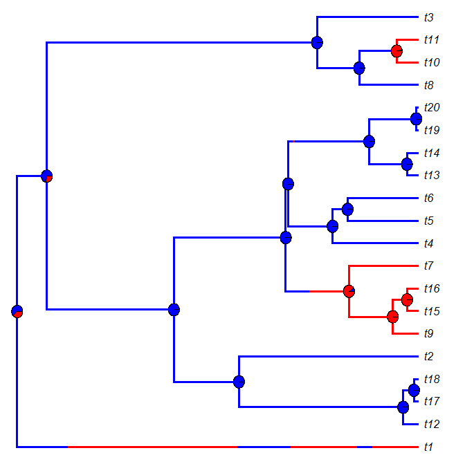
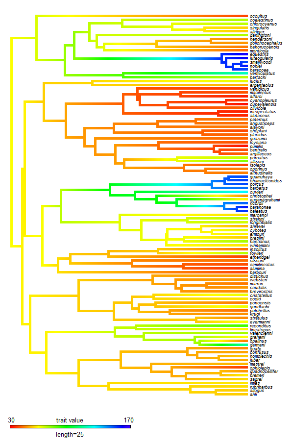
The phytools blog has also grown in popularity over the past year. Raw "pageview" counts can be affected by many things, and are thus difficult to interpret, but phytools blog has received over 90,000 pageviews since it's creation - over 60,000 in the past year. By any measure, that rate is growing - and this also equates to over 160 pageviews/day for 2012. Among the posts accruing the greatest number of pageviews in 2012: my series on xkcd style trees (e.g., 1, 2, 3); my entries on visualizing trait evolution on trees using colors (e.g., 1, 2); and my posts about ancestral character estimation under the threshold model from quantitative genetics (e.g., 1, 2, 3).

The phytools package (also on CRAN) has grown as well. From a small hodgepodge of methods, phytools has grown into a big one - now containing over 80 different functions and a PDF manual that (as of latest CRAN release) contained 87 pages.

Towards the end of 2012, phytools blog got a new look. Since when the original visual theme was created, phytools had no plotting functions (but now it has tons), this seemed appropriate. The blog also got a new URL (after I obtained the domain phytools.org).

I don't doubt for a second that 2013 will be just as productive as 2012 - so thanks for reading, and please keep coming back. Happy holidays!

Specifying pie colors in ancThresh & plotThresh

A phytools user contacted me to express difficulty in controlling pie colors at nodes using the new phytools functions for ancestral character estimation under the threshold model, ancThresh and plotThresh. This is done using the argument piecol, set to a vector with the states for the discrete trait as names, and the desired colors as values (in any format acceptable by R, e.g., here).

Here's a quick demo. I assume that we've already run the MCMC, and mcmc is the object returned by ancThresh. Data are in X:

> cols
   not     mod    high
"green"  "blue"   "red"
> plotThresh(tree,X,mcmc,piecol=cols,tipcol="estimated", label.offset=0.01)

Note that label.offset is on the scale of your phylogeny, so will have to be varied with total tree length. I've been meaning to migrate control of the pie sizes to the user, but have not yet had time to do so. (Plus, I've been sick.)

Plotting densityMap to PDF

A phytools user asks:
In the densityMap graphic you sent me it seemed like you had spread the branches apart some to make the tree more readable. Is that true? If so, could you tell me how?! I have attached a graphic I made and it looks terrible. . . .

Indeed it did look terrible.

In fact, there was really no mystery to how I used the same function to make a "nice" looking figure - I just used the 'grDevices' function pdf to plot directly to a PDF. This means I can set the dimensions of the plot to be anything I like, and squidged up branches and tip labels in an R plotting window will look nice!

Here's a quick example, using contMap (because densityMap is slow for large trees):

> tree<-pbtree(n=150)
> x<-fastBM(tree)
> pdf(file="contMap.pdf",height=14,width=5)
> # now the output of a plotting call will go to my PDF
> contMap(tree,x,outline=FALSE,fsize=c(0.6,1), lims=c(floor(range(x)[1]*10)/10,
ceiling(range(x)[2]*10)/10))
> # you can probably ignoring the "lims" argument
> # I've just used it here to get a nicer legend
> dev.off()
null device
          1

And here's the result (pulled from the PDF - obviously reduced in quality as a result):

New version of threshDIC

I just posted a new version of threshDIC for computing the Deviance Information Criterion from the object returned by ancThresh. The previous version (of threshDIC not ancThresh) just plain doesn't work. I made some mistakes on key calculations that are now fixed.

DIC is in some ways analogous to the Akaike Information Criterion (AIC), but provides the advantage that it can be used on the results of an MCMC chain - and thus doesn't not require that we can analytically or numerically solve for the maximum of the likelihood function.

The deviance is just -2 × the log-likelihood; and DIC requires that we calculate to versions of this - the mean deviance across samples (Dbar), and deviance at the mean parameter values from the posterior sample (Dhat. We penalize our IC by computing the effective number of parameters of the model (pD or pV, depending on the method we want to use).

Here's a quick demo for the dataset and tree I used earlier:

> require(phytools)
> threshDIC(tree,X,mcmc,sequence=c("not","mod","high"))
    Dbar      Dhat        pD       DIC
-21.29781 -68.07082  46.77302  25.47521

Just like with AIC, we should generally prefer the model with the lowest DIC - although DIC differences of less than 5-10 are difficult to interpret.

The new function is here, but I would advise downloading the latest version of phytools (phytools 0.2-15) and installing from source if you want to use this function:

> install.packages("phytools_0.2-15.tar.gz",type="source", repos=NULL)

Function setNames

I can't believe I just discovered the function setNames in the 'stats' package. All it is is a wrapper to combine the two lines of code required to create a vector & assign its names. (It can also be used to add names to other objects, such as a list.) So, for instance, instead of:

> x<-c(1:3)
> names(x)<-c("one","two","three")
> x
 one   two three
   1     2     3

We can do:

> x<-setNames(c(1:3),c("one","two","three"))
> x
 one   two three
   1     2     3

How have I been living without this for so long!

Faster inversion of square symmetric positive-definite matrices

For square, symmetric, positive-definite matrices (like covariance matrices) there is a method for faster matrix inversion that uses inversion of the Cholesky matrix. This is described here and implemented in the R package "Matrix". Here's a quick example, using the phylogenetic covariance matrix (vcv.phylo):

> require(phytools)
> # simulate tree
> tree<-pbtree(n=2000)
> C<-vcv(tree)
> # using solve
> system.time(Cinv1<-solve(C))
  user  system elapsed
 15.15    0.07   15.23
> system.time(Cinv2<-chol2inv(chol(C)))
  user  system elapsed
  6.69    0.02    6.74
> mean(abs(Cinv2-Cinv1))
[1] 3.953766e-16

That's faster.

Hypothesis testing using fitDiversityModel

A user had this question about using the function fitDiversityModel (which implements an ML version of the method in Mahler et al. (2010) to test hypotheses about phenotypic diversification:

I have one short question. In the paper by L. Mahler & al. they also tested the model with a single evolutionary rate. I’m asking me if it is “enough” to write it like that: Constant.time.results <- fitDiversityModel(tree,x,d=NULL)

The answer is "no" - but it is very easy to conduct the desired test. If fitDiversity(...,d=NULL), then the function estimates lineage density at each node as if the radiation is occurring within a single region (and there is no extinction or missing taxa - but that is a matter for another day); and then fits a model in which the rate of evolution varies as a function of lineage density. This will generally not be our null model. For that, we should specify d to be a vector of zeroes. We can then use a likelihood ratio test (for example) to test the null hypothesis that the pace of evolution has declined with increasing lineage density.

Here's a worked example, simulated so that the null is correct:

> require(phytools)
> # simulate tree & data under the null
> tree<-pbtree(n=100)
> x<-fastBM(tree)
> # fit the lineage-density model assuming a single region
> # (i.e., all contemporary ancestors were competitors)
> fitLD<-fitDiversityModel(tree,x)
no values for lineage density provided; computing assuming single biogeographic region
> fitLD
$logL
[1] -126.7954
$sig0
[1] 1.171704
$psi [1] -0.004116475
$vcv
            sig0           psi
sig0  0.121592376 -1.833989e-03
psi  -0.001833989  3.240988e-05

> # now fit the null hypothesis of constant rate
> d<-rep(0,tree$Nnode); names(d)<-1:tree$Nnode+length(tree$tip)
> fitNull<-fitDiversityModel(tree,x,d)
psi not estimable because diversity is constant through time.
> fitNull
$logL
[1] -127.0581
$sig0
[1] 0.9602251
$vcv
            sig0
sig0 0.01844064

> # now test using LR
> LR<-2*(fitLD$logL-fitNull$logL)
> P<-pchisq(LR,df=1,lower.tail=F)
> P
[1] 0.4685722

The null model is just pure Brownian motion; and we would obtain the same parameter estimate and likelihood using, say, fitContinuous in the geiger package:

> fitContinuous(tree,x)
Fitting BM model:
$Trait1
$Trait1$lnl
[1] -127.0581
$Trait1$beta
[1] 0.9602253
$Trait1$aic
[1] 258.1161
$Trait1$aicc
[1] 258.2411
$Trait1$k
[1] 2

That's it.

Plotting node piecharts on top of a plotSimmap tree

Today a user asked:

I was wondering: is it possible to use nodelabels(pie=data,cex=0.4) from ape to draw piecharts on top of the plotSimmap (at nodes)? I've tried a bit with the default settings, but it didn't do a good job with placing piecharts at correct nodes. Changing margins didn't help too.

plotSimmap and plot.phylo use totally different coordinate systems; in addition, plot.phylo returns its settings invisibly to the environment - settings that are in turn used by helper functions like nodelabels. Consequently, I expected that this would be impossible, or at least difficult. As it turns out, it is only the latter (i.e., difficult, not impossible).

The solution (a hack) relies on two key ingredients: transforming the SIMMAP trees to the scale that is used internally by plotSimmap; and, secondly, first calling plot.phylo(...,plot=FALSE), which opens a plotting device and tells R a tree has been plotted, even though one has not. The rest, I figured out by tinkering!

Here is the solution - by way of simulated example. Within this example, I also show how to compute the relative frequency of node states in a set of stochastic mapped trees (after all, what else would we want to plot at internal nodes):

# code to simulate a tree & data
# and to perform stochastic mapping
tree<-pbtree(n=20)
Q<-matrix(c(-1,1,1,-1),2,2)
colnames(Q)<-rownames(Q)<-c(0,1)
x<-sim.history(tree,Q,anc="0")$states
mtrees<-make.simmap(tree,x,nsim=100)
# end simulation code

# function to compute the states
foo<-function(x){
  y<-sapply(x$maps,function(x) names(x)[1])
  names(y)<-x$edge[,1]
  y<-y[as.character(length(x$tip)+1:x$Nnode)]
  return(y)
}
XX<-sapply(mtrees,foo)
pies<-t(apply(XX,1,function(x,levels,Nsim) summary(factor(x,levels))/Nsim,levels=c("0","1"),Nsim=100))
# done computing the states

# code to plot the tree
mtrees<-rescaleSimmap(mtrees,1)
cols<-c("blue","red"); names(cols)<-c(0,1)
par(mar=rep(0.1,4))
plot.phylo(mtrees[[1]],plot=FALSE,no.margin=T)
plotSimmap(mtrees[[1]],cols,pts=FALSE,lwd=3,ftype="off", add=TRUE)
text(1,1:length(mtrees[[1]]$tip),mtrees[[1]]$tip.label, pos=4,font=3)
nodelabels(pie=pies,cex=0.6,piecol=cols)
# done plotting

And here is the result of one such simulation & plotting exercise:

For fun, let's compare this to densityMap:

> densityMap(mtrees,lwd=6)
sorry - this might take a while; please be patient

Cool.

"Recent Comments" widget back

For a few weeks the blogger.com "Recent Comments" gadget has been broken so I pulled it from my sidebar. Today I decided to track down some 3rd party code and "Recent Comments" is back online! (See the sidebar.) Comments are always appreciated & welcome (and at least as likely to get a quick response as an email - which, unfortunately, is not as likely as I'd wish).

Ancestral character estimation under the threshold model: an example

I just posted a new version of the phytools function ancThresh for ancestral character estimation using the threshold model from quantitative genetics. Under the threshold model evolution is of an unknown, and unobserved, continuous character, "liability." When liability exceeds a particular value (the threshold or one of multiple thresholds) the observed, discretely valued character trait changes state. (See the following link for much more discussion of the threshold model on this blog.)

The most significant change from prior versions of the function is that the present version can accept either a vector of length N containing a fixed set of trait values for the tips (as before) or a matrix of dimension N × m (for m conditions of the discrete character) in which the i,jth element contains the prior probability of tip i being in state j. This is not equivalent to modeling within-species polymorphism. Rather we allow the possibility that a tip state is unknown, or that it can be called in one condition or another with definable probability.

I have also added the function plotThresh. This function plots the posterior probabilities of ancestral states on the tree. It is called internally (by default) in ancThresh - but also can be called on its own and given the posterior sample from an MCMC run.

Here's a quick example using the phylogeny of Centrarchidae in Near et al. (2005) and the data for feeding mode (including uncertainty) from Collar et al. (2009). Note that for taxa missing from the Collar et al. study I have assigned states for feeding mode based on the behavior of close relatives - I could have equally well decided that feeding mode was unknown for those species.

> tree<-read.tree("Centrarchidae.tre")
> X<-read.csv("Centrarchidae.csv",header=T,row.names=1)
> X
                           not    mod   high
Acantharchus_pomotis     0.0000 1.0000 0.0000
Lepomis_gibbosus         1.0000 0.0000 0.0000
Lepomis_microlophus      1.0000 0.0000 0.0000
Lepomis_punctatus        1.0000 0.0000 0.0000
Lepomis_miniatus         0.5000 0.5000 0.0000
...
Ambloplites_ariommus     0.3333 0.3333 0.3333
...
> mcmc<-ancThresh(tree,X,ngen=1000000,control= list(piecol=cols,tipcol="estimated"),label.offset=0.01)
**** NOTE: no sequence provided, column order in x
MCMC starting....
gen 1000
gen 2000
....
> layout(c(1,2),heights=c(0.9,0.1))
> plotThresh(tree,X,mcmc,piecol=cols,tipcol="estimated", label.offset=0.01)
> plot.new()
> plot.window(xlim=c(0,10),ylim=c(-2,1.25))
> points(0.2,1,pch=19,col="green",cex=2)
> text(0.2,1,"non-piscivorous",pos=4,offset=0.7)
> points(0.2,0,pch=19,col="blue",cex=2)
> text(0.2,0,"moderately piscivorous",pos=4,offset=0.7)
> points(0.2,-1,pch=19,col="red",cex=2)
> text(0.2,-1,"highly piscivorous",pos=4,offset=0.7)

Note that plotThresh(...,tipcol="estimated") uses the sampled liabilities for tips from the MCMC to obtain posterior probabilities for the trait values of uncertain tips. I could also using plotThresh(...,tipcol="input") to get back the input probabilities.

Well, that's pretty cool. Since there are whole bunch of helper functions that are called internally by ancThresh and plotThresh, I would strongly advise installing the latest minor phytools build (phytools 0.2-14) - rather than loading the source code directly - if you are interested in repeating the analyses of this post. Word of caution (!) - ancThresh is still in very early development (and should be treated as such).

Plot outline-only tree

I realized after posting yesterday that the same trick could be used to plot a pure "outline" tree (i.e., white edges outlined in black). Here's how, using the centrarchid tree of Near et al. (2005):

> # set line widths
> lwd.outer=9; lwd.inner=5
> par(col="white") # font color white
> plotTree(tree,lwd=lwd.outer,ftype="i")
> par(col="black") # reset
> # now the tricky part: create a "fake" mapping
> maps<-tree$edge.length
> maps<-as.list(maps)
> for(i in 1:length(maps)) names(maps[[i]])<-"1"
> cols<-"white"; names(cols)<-"1"
> tree$maps<-maps
> plotSimmap(tree,cols,lwd=lwd.inner,pts=F,add=T,ftype="i", offset=0.2*lwd.outer/3+0.2/3)

That's it.

Plotting an outline around a stochastic character mapped tree

In the functions contMap and densityMap I introduced the option of "outlining" the plotted edges with a fine black line (e.g., described here). It is also now possible to do this with typical stochastic mapped trees using plotSimmap, although not as a built-in option. Here's a quick demo (illustrated with simulated data):

> # first simulate tree & data
> Q<-matrix(c(-2,1,1,1,-2,1,1,1,-2),3,3)
> tree<-sim.history(pbtree(n=30,scale=1),Q,anc=1)
> # now plot (modify as desired
> cols<-c("blue","red","green"); names(cols)<-1:3
> lwd.outer=9; lwd.inner=5
> par(col="white") # font color white
> plotTree(tree,lwd=lwd.outer,ftype="i")
> par(col="black") # reset
> plotSimmap(tree,cols,lwd=lwd.inner,pts=F,add=T,ftype="i", offset=0.2*lwd.outer/3+0.2/3)

What we're doing here is not complicated. Basically, the option plotSimmap(...,add=TRUE) (new only in the latest versions of phytools) lets us first create a tree with the edges plotted in plain black; onto which we overlay the slightly finer lines of our plotted stochastic character mapped tree. A neat thing about this technique is that we use white as a mapping color and it doesn't look ridiculous, for instance, using the same tree as before:

> cols<-c("white","red","green"); names(cols)<-1:3
> lwd.outer=9; lwd.inner=5
> par(col="white") # font color white
> plotTree(tree,lwd=lwd.outer,ftype="i")
> par(col="black") # reset
> plotSimmap(tree,cols,lwd=lwd.inner,pts=F,add=T,ftype="i", offset=0.2*lwd.outer/3+0.2/3)

Finally, readers might notice that to specify the outer line widths, I have added a specifically even number to the inner line width (here, 4 - but it could be 2 or 6). This results in the appearance of a line of equal thickness on either side of the plotted tree. If we use an odd number instead, the appearance is a slight shadow. For instance - readers can try the code below:

> cols<-c("blue","red","green"); names(cols)<-1:3
> lwd.outer=9; lwd.inner=6
> par(col="white") # font color white
> plotTree(tree,lwd=lwd.outer,ftype="i")
> par(col="black") # reset
> plotSimmap(tree,cols,lwd=lwd.inner,pts=F,add=T,ftype="i", offset=0.2*lwd.outer/3+0.2/3)

(although there are probably better ways to generate a more pronounced shadow - perhaps the subject of a future post).

New minor phytools version (v0.2-13)

I also just built and posted a new minor phytools version (v0.2-13). The source code can be downloaded here.

This version includes the following over the last minor release:
1. Minor bug fixes to densityMap.
2. New functions roundBranches and applyBranchLenghts (see code here).
3. Minor bug fix for rescaleSimmap to correctly handle a "multiPhylo" object.

As well as the following updates of the last major phytools release (v0.2-1):
4. Various major bug fixes to phyl.RMA.
5. New function for plotting a tree in multiple columns, splitplotTree.
6. New function for adding a tip to the tree, bind.tip.

To install, download the package source, and then:

> install.packages("phytools_0.2-13.tar.gz",type="source", repos=NULL)
* installing *source* package 'phytools' ...
** R
...
* DONE (phytools)

That's it!

Issue with plotting output trees from SIMMAP using densityMap

A phytools user contacted me yesterday with the following issue:

I was trying to use your densityMap function to visualize some output from SIMMAP. The mutational mappings seemed to work fine in SIMMAP. I tried importing into R using read.simmap, this seemed to work fine. I then tried to use densityMap but it keeps giving me the following error:
> trees<-read.simmap(file)
> densityMap(trees,res=1000)
sorry - this might take a while; please be patient
Error in lower:upper: NA/NaN argument

This isn't something that I'd seen before, but I recognized that the code is from a part of the function in which the beginning and ending points for each map segment on a branch (XX) is compared to a matrix containing the beginning and ending points for every step interval along the same edge (YY); in which these steps are based on the edge length of the branch and the function argument res. Importantly, the beginnings and endings are in terms of the height above the root.

This made me suspect that the problem was with the edge lengths of the tree. densityMap assumes that the topology of the input trees are equal with proportional branch lengths. (In fact, there is an option - densityMap(...,check=TRUE) - that evaluates this equality criterion, and returns an error message if it fails.) For some reason that I don't completely understand (and even when 'mutational mapping' is performed on a single input tree), SIMMAP returns a sample of trees with varying total length. Theoretically, this should not be a problem if the branch lengths are strictly proportional. Unfortunately, due to numerical precision (which is relatively low - 6 digit - in the SIMMAP output), the branch lengths of these varyingly scaled trees are not strictly proportional. Consequently, even after they have been scaled to the same total length using phytools function rescaleSimmap (which is done internally in densityMap), the trees have slightly different branch lengths - sufficiently different, evidently, to account for this error.

My eventual workaround was to write a function that would apply one set of branch lengths (say, from a reference tree) to another tree or set of trees. For basic "phylo" objects, this is trivial of course. We would just do:

# for reference tree tr1
tr2$edge.length<-tr1$edge.length

However, for trees with mappings, it is slightly more complicated. Here is a simplified version of the function:

applyBranchLengths<-function(tree,edge.length){
  if(class(tree)=="multiPhylo"){
    trees<-lapply(tree,applyBranchLengths,
      edge.length=edge.length)
    class(trees)<-"multiPhylo"
    return(trees)
  } else {
    tree$edge.length<-edge.length
    if(!is.null(tree$maps)){
      for(i in 1:nrow(tree$edge)){
        temp<-tree$maps[[i]]/sum(tree$maps[[i]])
        tree$maps[[i]]<-temp*tree$edge.length[i]
      }
    }
    return(tree)
  }
}

This function uses the proportional time spent in each state along each edge of the target tree in rescaling the mappings to the reference tree. (I've left out calculation of the $mapped.edge matrix here, which involves a few more lines of code.) I have posted the full function code for this here.

Anyway, it worked! Here's a quick demo with a simulated tree & dataset in which I performed stochastic mapping using SIMMAP v1.5 for another project:

> trees<-read.simmap("simmap.trees.nex",format="nexus", version=1.5)
> densityMap(trees)
sorry - this might take a while; please be patient
Error in lower:upper : NA/NaN argument
> # get the tree heights
> h<-sapply(trees,function(x) max(nodeHeights(x)))
> h
 [1] 13.215321  6.213479 16.864350  9.936482 ....
 ...
> # ok, they have different heights - is that the problem?
> # try rescaling
> rescaled<-rescaleSimmap(trees,mean(h))
> densityMap(rescaled)
sorry - this might take a while; please be patient
Error in lower:upper : NA/NaN argument
> # nope!
> # ok, how about *not* rescaling, but applying the
> # relative branch lengths from trees[[1]] to all the
> # trees in the sample
> newbl<-mapply(applyBranchLengths,trees, lapply(as.list(h),"*",trees[[1]]$edge.length/h[1]), SIMPLIFY=FALSE)
> class(newbl)<-"multiPhylo"
> # these trees have their original total lengths
> # but relative branch lengths from trees[[1]]
> densityMap(newbl,fsize=c(0.6,1))
sorry - this might take a while; please be patient

Plotting many stochastically mapped trees

I recently described a new function, densityMap (1, 2), that can be used to plot the posterior probability of a binary trait evolving along the branches of the tree based on the method of stochastic character mapping (Neilsen 2002; Huelsenbeck et al. 2003; Bollback et al. 2006). There's another way to do this, of course - we can just plot them all! Here's a quick demo & the resultant visualization (from 100 stochastic maps):

> # data for the binary [0,1] state in x
> trees<-make.simmap(tree,x,nsim=100)
> par(mfrow=c(10,10))
> cols<-c("blue","red"); names(cols)<-c(0,1)
> plotSimmap(trees,cols,ftype="off",lwd=1,pts=F)

That's pretty cool. Still, I think there is an argument for densityMap:

> par(mfrow=c(1,1))
> densityMap(trees)
sorry - this might take a while; please be patient
Waiting to confirm page change...

Fitting the λ model in phylogenetic regressions using various functions

A R-sig-phylo reader recently asked the following:

I am trying to implement Liam Revell's suggestion on the evaluation of Pagel's lambda simultaneous to fitting PGLS to minimize the effects of wrong model selection (OLS vs. PGLS) on species data (i.e. Revell 2010, Methods in Ecology and Evolution 1: 319-329).Does anyone know if this kind of simultaneous optimization of lambda and PGLS parameters is presently implemented in R? The obvious place would be phytools, but I could not find anything similar in that package.

In fact, this is possible using multiple functions in several packages. Unfortunately, it is not always completely obvious - so the question is (in my opinion) fully justified! Specifically, this can be done using nlme::gls, caper::pgls, and (indeed) phytools::phyl.resid. Here's my summary (modified from my response) of how (which I repeat here in the hope that it will help folks in future when they are searching for information on this topic):

# using ape & nlme
library(ape); library(nlme)
# assuming your data are contained in named vectors x & y
y<-y[names(x)]
fit<-gls(y~x,data.frame(x,y),correlation=corPagel(1,tree, fixed=FALSE),method="ML")
# assuming your data are in data frame X, with column names
# var1, var2, etc.; for example:
fit<-gls(var1~var2+var3,X,correlation=corPagel(1,tree, fixed=FALSE),method="ML")

# using caper
library(caper)
# assuming your data are in named vectors x & y
y<-y[names(x)]
X<-data.frame(x,y,Species=names(x))
fit<-pgls(y~x,comparative.data(tree,X,"Species"), lambda="ML")

# using phytools
library(phytools)
# assuming your data are in named vectors x & y
fit<-phyl.resid(tree,x,y,method="lambda")

I would generally recommend using gls & pgls over phyl.resid, because they "play well" with generic functions such as summary and residuals, with the following caveats (1) phyl.resid may be a little easier to use (because it takes standard arguments, no functions or formulae); and (2) phyl.resid (for some reason) seems to run a little faster, especially for large trees. (For instance, it took only 45s on a tree with 1000 tips while gls took over a minute and pgls over 4 minutes. This could be important for investigators repeating the same analysis on many trees - for instance, a sample from the posterior distribution of a Bayesian phylogeny inference run.)

Update to function matchNodes

I'm working on a manuscript review this Saturday and (I don't think I'm giving away too much about the article to say that) I needed a function to match the node numbers of a tree with the same nodes in a re-rooted version of the same phylogeny. This differs from the purpose of my previous phytools utility function, matchNodes, which matches nodes based on the commonality of their descendant tips. This method will not, in general, produce the correct set of matchings for a tree that has merely been rerooted at an internal node.

My idea for obtaining the correct matchings was to use the set of distances to the tip species in the tree. Matching nodes with the same set of patristic distances (or, for trees with arbitrary scale, proportional distances) must be equivalent. Here is the core code of the function:

D1<-dist.nodes(tr1)[1:length(tr1$tip), 1:tr1$Nnode+length(tr1$tip)]
D2<-dist.nodes(tr2)[1:length(tr2$tip), 1:tr2$Nnode+length(tr2$tip)]
rownames(D1)<-tr1$tip.label
rownames(D2)<-tr2$tip.label; D2<-D2[rownames(D1),]
for(i in 1:tr1$Nnode){
  z<-apply(D2,2,function(X,y) cor(X,y),y=D1[,i])
  Nodes[i,1]<-as.numeric(colnames(D1)[i])
  Nodes[i,2]<-as.numeric(names(which(z>=(1-tol))))
}

The first part of the code uses the 'ape' function dist.nodes to compute the set of distances from each node to all tips; and then sorts them to have the same row-wise ordering in the two matrices. Next, we go through the columns of D1 and identify the column of D2 with proportional or equal distances.

Of course - some important bookkeeping has been omitted here. For the full code, see utilities.R on the phytools page.

Let's try it out:

> tr1<-pbtree(n=20)
> par(mfcol=c(1,2))
> plotTree(tr1,node.numbers=T)
> # re-root tr1 at node=33
> tr2<-root(tr1,node=33)
> plotTree(tr2,node.numbers=T)

> matchNodes(tr1,tr2,method="distances")
      tr1 tr2
[1,]  21  NA
[2,]  22  30
[3,]  23  31
[4,]  24  32
[5,]  25  29
[6,]  26  25
[7,]  27  26
[8,]  28  27
[9,]  29  28
[10,]  30  24
[11,]  31  23
[12,]  32  22
[13,]  33  21
[14,]  34  38
[15,]  35  33
[16,]  36  34
[17,]  37  35
[18,]  38  36
[19,]  39  37

> # we can also reverse the order of the trees
> matchNodes(tr2,tr1,method="distances")
      tr1 tr2
[1,]  21  33
[2,]  22  32
[3,]  23  31
[4,]  24  30
[5,]  25  26
[6,]  26  27
[7,]  27  28
[8,]  28  29
[9,]  29  25
[10,]  30  22
[11,]  31  23
[12,]  32  24
[13,]  33  35
[14,]  34  36
[15,]  35  37
[16,]  36  38
[17,]  37  39
[18,]  38  34

Careful inspection of the matchings above should (I hope) reveal that the nodes from tr1 have been correctly matched to the corresponding nodes of tr2 (in the first example - and the converse in the second case). The column headings in the second example reflect the input order of the trees - not their names in memory.

Note that case 1 leaves one unmatched node - the root. In case two there are no unmatched nodes because all of the n - 2 nodes in tr2 have a compatriot in tr1.

Assuming no major errors are identified, this function will be in the next version of phytools.

That's it.

New minor phytools version 0.2-11

I just posted a new minor package update (phytools 0.2-11). It can be downloaded here and installed from source. This new version has a small number of significant updates and new functions:

1. A new function (splitplotTree, also see inset) to split a plotted tree into multiple columns or plotting windows, along with one minor bug fix.

2. A couple of important bug fixes for phyl.RMA, my function for phylogenetic RMA (1, 2).

3. Finally, a new function, bind.tip, for attaching a new species to the tree (1, 2). If no terminal edge length is provided the function automatically checks to see if the tree is ultrametric and (if it is) scales the terminal edge length so that ultrmetricity is maintained.

To install from source, just download the build and then type:

> install.packages("phytools_0.2-11.tar.gz",type="source", repos=NULL)

at the R prompt. Good luck!

Bug fix for phyl.RMA

A user pointed out that phyl.RMA did not work (specifically, returned the incorrect signed RMA slope) when the relationship between x & y is negative. This is, in fact, correct. I have now fixed this problem by changing the following line of code:

beta1<-sqrt(temp$R[2,2]/temp$R[1,1])

to:

beta1<-sign(temp$R[1,2])*sqrt(temp$R[2,2]/temp$R[1,1])

the difference being that in the latter case I pre-multiply the evolutionary variance ratio by the sign of the interspecific covariance. Updated code is here and will be in the next version of phytools.

This update introduces the problem that our statistic for hypothesis testing the RMA regression slope, based on equation [8] of McArdle (1988), is only defined for positive RMA regression slopes. To address this, I have boldly assumed that for h₀: β < 0 the null distribution is symmetric about 0 & consequently if b & β have the same sign, I use equation [8] on the absolute values of b & β - otherwise I set T to zero & return a warning. This (at least) has the desirable effect of using McArdle equation [8] without modification with b and β are both > 0 (typical of hypothesis tests about allometry).

Note that, unlike in LS regression, for RMA we cannot normally test h₀: β = 0. This is because β = 0 implies that σ_y = 0.

Testing for Pagel's λ < 1.0

A recent commenter on the phytools blog asks:
I’m working on a comparative phylogenetic project and want to show that my data has phylogenetic signal. Using Pagel’s lambda I get lambda – 0.854. Is this value significant enough in that it’s safe to model the variable as Brownian motion?

I interpret this to mean "how can we test the alternative hypothesis that Pagel's λ is less then 1.0; against the null that λ=1.0." This is easy if we accept the contention that our likelihood ratio should be distributed as a Χ² with 1 degree of freedom (for one parameter, λ, estimated in the more complex model), an asymptotic property of likelihoods. (There may be some very good reasons - which we'll set aside for the moment - to question this assertion, for instance see a recent article by Carl Boettiger et al.)

This can be done most naturally using the fitContinuous function in 'geiger' - but we can also do it using entirely phytools functions, and since I developed and maintain phytools (not geiger), I'll demo that option.

First, let's simulate a tree & data for the demo, using the λ=0.854 obtained by the commenter. We will use geiger::lambdaTree for this part:

> library(phytools); library(geiger)
> # simulate tree
> tree<-pbtree(n=50)
> # simulate data with lambda=0.854
> x<-fastBM(lambdaTree(tree,0.854))

OK, now let's fit both models, compute the likelihood ratio, and then compare it to a Χ² distribution with one degree of freedom. We need to use a little bit of a work-around to fit the BM model using brownie.lite:

> # fit lambda model
> lambda<-phylosig(tree,x,method="lambda")
> lambda
$lambda
[1] 0.9497926
$logL
[1] -87.54412
> # get likelihood for bm model
> tree$mapped.edge<-matrix(tree$edge.length, nrow(tree$edge),1,dimnames=list(NULL,"1"))
> bm.logL<-brownie.lite(tree,x)$logL1
> # conduct hypothesis test using chi-square
> LR<--2*(bm.logL-lambda$logL)
> P<-pchisq(LR,df=1,lower.tail=F)
> P
[1] 0.1346832

So, in this simulated case at least, we cannot distinguish our estimated phylogenetic signal from Brownian motion.

An additional word of caution, however. Sampling error in the estimation of species means can also have the effect of depressing phylogenetic signal - so if the species means are estimated with a limited number of samples per species, it might be wise to conduct this analysis including estimated within species sampling variances. These can be supplied using the argument se in both phylosig and brownie.lite.

Addendum to adding a single tip to the tree

Yesterday I posted an extremely simple function for adding an extra tip to the tree. In response to a user request, here is an addendum in which the function also checks if the tree is ultrametric and (so long as a custom branch length is not supplied) computes a branch length for the added tip such that the tree remains ultrametric after the new tip is added. Since this wraps around the 'ape' function bind.tree, I have also added the argument position, which is the distance below the specified node where the new tip should be added. First, here's the function:

bind.tip<-function(tree,tip.label,edge.length=NULL, where=NULL,position=0){
  if(is.null(where)) where<-length(tree$tip)+1
  if(is.null(edge.length)&&is.ultrametric(tree)){
    H<-nodeHeights(tree)
    if(where==(length(tree$tip)+1))
     edge.length<-max(H)
    else
     edge.length<-max(H)-H[tree$edge[,2]==where,2]+position
  }
  tip<-list(edge=matrix(c(2,1),1,2),
    tip.label=tip.label,
    edge.length=edge.length,
    Nnode=1)
    class(tip)<-"phylo"
  obj<-bind.tree(tree,tip,where=where,position=position)
  return(obj)
}

And here's a demo:

> tree<-pbtree(n=10)
> plotTree(tree,node.numbers=T)

> # now add 1/2 branch length below node 16
> tree2<-bind.tip(tree,"t11",where=16, position=0.5*tree$edge.length[which(tree$edge[,2]==16)])
> plotTree(tree2,node.numbers=T)

Cool - it works.

Note that if we want to add a new terminal edge along a branch leading to a tip - we have to specify the tip by node number not tip label. So, for instance, to add another tip to our new tree halfway along the branch leading to tip t11, we would do:

> tree3<-bind.tip(tree2,"t12",
 where=which(tree2$tip.label=="t11"),
 position=0.5*tree2$edge.length[which(tree2$edge[,2]==
 which(tree2$tip.label=="t11"))])
> plotTree(tree3,node.numbers=T)

Adding a single tip to a tree

A R-sig-phylo member writes:

Dear list members,
I have a large phylogeny to which I need to add branches of a certain length (new taxa) at specific nodes.
I have experimented with bind.tree (ape) and paste.tree (phytools) but they only let you bind trees to together. I can cobble together code that adds a 2 species tree and then erase one of the tips using drop.tip but this is difficult given how the node labels change.
I want to automate this process because I have ~180 additions to make and I want to repeat the additions using branches of different length.
Ideally I would like to have a function where I input the node number to which a branch should be added, the length of that branch, and the name of the tip.
Any suggestions?

It seems like the basic problem is not that bind.tree and paste.tree don't work; but rather that they only attach two bifurcating trees together, and the user wants to attach one tip to a tree.

Well, it turns out that this is not too hard. Here's how, by way of demonstration:

> library(phytools)
> # simulate receptor tree
> tree<-pbtree(n=10)
> plotTree(tree,node.numbers=T)

> # create tip (modify as desired)
> tip<-list(edge=matrix(c(2,1),1,2),
    tip.label="species.name",
    edge.length=1.0,
    Nnode=1)
> class(tip)<-"phylo"
> # attach to any node (say, node 16)
> btree<-bind.tree(tree,tip,where=16)
> plotTree(btree)

Ok, how about writing a function for it? Let's call it bind.tip:

bind.tip<-function(tree,tip.label,edge.length=NULL,where=NULL){
  if(is.null(where)) where<-length(tree$tip)+1
  tip<-list(edge=matrix(c(2,1),1,2),
    tip.label=tip.label,
    edge.length=edge.length,
    Nnode=1)
  class(tip)<-"phylo"
  obj<-bind.tree(tree,tip,where=where)
  return(obj)
}

That's it.

Function to break up plotted tree into multiple columns of figures

In early October, a R-sig-phylo query was submitted that read as follows:

I'm wondering if there is a way to plot a phylogeny in R that is broken up and displayed side by side to condense space. I've made a backbone in R that i'd like to make into a figure, but it is too tall. If this isn't the write setup, could someone suggest what program (and format for me to write.tree) from R. I am using windows, in terms of potential third part programs.

Well, I thought this sounded like a neat idea. We often see trees plotted this way in published articles, but there is no native function in R to produce this kind of plot. Unfortunately, I didn't have time to work on this until recently - so most likely, the author of the R-sig-phylo question has already solved this problem in some other way. Nonetheless. . . . .

(I should note that, in discussing this function with my friend Luke Harmon, he warned me that I was stuck in the "paper paradigm" - for more on what that means, see Luke's article with James Rosindell.)

Ignoring Luke (as is my wont), I just posted a function for this anyway. The function, splitplotTree, can be downloaded from my phytools page (direct link to code here).

A little bit about how I did this. . . . To plot a phylogram we need two coordinate matrices: a matrix for the heights of the nodes above the root; and a matrix for the vertical position of the edges. We get the former for a "phylo" object by using (say) nodeHeights in phytools. To get the latter, we can just evenly space the tip nodes on our vertical axis (for a rightward facing tree); and then work down through their common ancestors to the root, averaging the vertical position of the descendant nodes to obtain the height of each parent.

Having done this, to split the tree horizontally we just have to select a cutting point. Then we split our matrices based on this point. After some adjustments, we plot our trees in each plot window. Finally, we have to plot the vertical lines (the lines connecting daughter edges) that would normally connect the two plots. This is easy. For the upper panel tree slice, we just plot a line from each unmatched node to the lower edge of the plot; and for the lower panel tree, we do the opposite. The result will look something like this:

> library(phytools)
> source("splitplotTree.R")
> tree<-pbtree(n=100)
> splitplotTree(tree,fsize=0.7,ftype="i",split=0.5)

We might look at this and decide that we don't like the look of the slice point split and would prefer to break the tree, say, between tips t76 and t43. After some fiddling, we can figure out where that split point needs to be:

> splitplotTree(tree,fsize=0.7,ftype="i",split=0.54)

Note that the vertical position of the tree is automatically adjusted so that the spacing of the tips is equal in both panels.

If we would rather plot our tree in two windows, rather than in side-by-side panels (say, for publication across two journal pages), we can do that too.

> splitplotTree(tree,fsize=0.7,ftype="i",split=0.54, new.window=TRUE)

Panel 1:

and panel 2:

Finally, the function can also be used to create a silly (and, so far as I know, entirely useless) animation of a tree gradually sliding from one side of a plotting window to another. Here, for the Greater Antillean anole tree:



And the code used to do this (minus functions for saving frames to movie file for external viewing):

# code for animation
layout(matrix(c(1,2),1,2))
plotTree(anoletree,fsize=0.7,ftype="i"); layout(1)
for(i in 198:2) splitplotTree(anoletree,split=i/200,fsize=0.7,ftype="i")
layout(matrix(c(2,1),1,2))
plotTree(anoletree,fsize=0.7,ftype="i"); layout(1)

That's it!

Bug fix for phyl.RMA

I recently received the following bug report for the phytools function for reduced major axis regression (phyl.RMA):

I've been encountering an error when trying to run phyl.RMA:

Error in D %*% t(a) : non-conformable arguments
In addition: Warning message:
In if (lambda == 1) return(C) else { :
the condition has length > 1 and only the first element will be used

What's odd is that with R 2.15.1 and the previous version of phytools, it ran perfectly. But today I updated to R 2.15.2 and the latest version of phytools, and it's a no-go. Any idea what's going on here?

Indeed - I can reproduce this error easily:

> require(phytools)
Loading required package: phytools
...
> tree<-pbtree(n=100)
> x<-fastBM(tree)
> y<-fastBM(tree)
> args(phyl.RMA)
function (x, y, tree, method = "BM", lambda = NULL, fixed = FALSE,
    h0 = 1)
NULL
> phyl.RMA(x,y,tree)
Error in D %*% t(a) : non-conformable arguments
In addition: Warning message:
In if (lambda == 1) return(C) else { :
  the condition has length > 1 and only the first element will be used

Turns out, though, that the association with R 2.15.2 is completely spurious. The real problem came when I moved the code for various utility functions out of the functions that used them, such as phyl.pca, phyl.cca, and, lo & behold, phyl.RMA. As it turned out, some of the argument list order differed between different iterations of internally called functions (the culprit in this case was lambda.transform).

I have fixed the problem, and the revised function (here) seems to work:

> source("phyl.RMA.R")
> phyl.RMA(x,y,tree)
$RMA.beta
[1] 0.06725208 0.86425086
$V
           x          y
x 0.93872556 0.06935903
y 0.06935903 0.70116186
$lambda
[1] 1
$logL
[1] -264.4581
$test
        r2           T          df           P
0.00730885  1.44956623 99.64317035  0.15031966
$resid
              [,1]
t39  -0.2958474582
t40   0.5487124406
t9    ...

Good.

New version of phytools (0.2-1) on CRAN

There is a new version of phytools on CRAN (phytools 0.2-1). This can be downloaded and installed from source from the CRAN or from the phytools webpage. It should also be available for installation using install.packages("phytools") some time in the next few days as the Mac OS and Windows binaries are built and phytools 0.2-1 percolates through the CRAN mirrors.

I have made a few small updates, mostly to documentation, from the last minor (non-CRAN) package version, phytools 0.2-05, but otherwise it is the same. There are lots of updates of note, though, with respect to the previous CRAN release (phytools 0.2-0). Here's a list of the major items:

1. A new function (fastAnc) for fast ML ancestral state estimation (1, 2).

2. A new function (matchNodes) to match nodes between trees.

3. A new function (xkcdTree) to plot xkcd style phylogenetic trees (1, 2, 3, 4, 5, 6, 7). xkcdTree can also be called from within fancyTree.

4. A new Bayesian MCMC method (ancThresh) for ancestral character estimation under the treshold model (1, 2, 3, 4).

5. A new function (multi.mantel) for multiple matrix regression with Mantel test (i.e., "partial Mantel tests").

6. A new method and function (densityMap) for visualizing the posterior density from stochastic mapping on the tree (1, 2).

7. Finally, a new function (contMap) for plotting the reconstructed values of a continuously valued trait on the tree (1, 2).

The phytools R package now contains over 80 different function and an 87 page PDF manual. Yikes!

New URL

The phytools blog has a new URL: blog.phytools.org. This should not affect the way readers experience the phytools blog, and all old links with the phytools.blogspot.com URL should be unaffected.

In addition, the URL www.phytools.org should automatically redirect to the phytools development page.

Thanks for reading!

Update to the visual theme of the blog

After nearly two years and over 300 posts, I decided to make some minor changes to the theme & background of the blog. The most obvious one is the the updated background image & color (reproduced here at right).

Since the original background image (a radial tree with a multicolored stochastic mapping) was created before phytools had any graphical functions (and, in fact, before the package formally existed), I thought the update was overdue. The new images were created using densityMap and contMap with some very minor post-hoc editing.

Code for contMap & new minor phytools version

I just posted the code for contMap, a new phytools graphing function for plotting the reconstructed value of a continuous character along ancestral branches and nodes in the tree (previously described here). I made a couple of updates to the function, including some changes that allow the user to specify the trait range of the legend (previously the default was just the range of extant phenotypes). I have also built a new minor (i.e., non-CRAN) version of phytools, v0.2-05, which can be downloaded here and installed from source. Note that I have a submitted manuscript describing this function and densityMap (1, 2). See help(contMap) for citation information.

Here's a quick demo, including installation from source, again, with the Greater Antillean Anolis tree and data for SVL (data & tree not included):

> install.packages("phytools_0.2-05.tar.gz",type="source", repos=NULL)
* installing *source* package 'phytools' ...
...
* DONE (phytools)
> library(phytools)
Loading required package: ape
...
> contMap(anoletree,svl,res=200,fsize=c(0.6,0.8),outline=F, lims=c(30,170),lwd=5)

**Note, the difference between this figure and a prior iteration is because trait values are on mm rather than log(mm) scale; and I have rescaled the total tree length to 50 Ma - based on a very approximate age for the root of Greater Antillean anoles of 50 mybp (and following Mahler et al. In review).

Mapping the reconstructed value of a quantitative character on the tree

Following my new function, densityMap, for mapping the posterior density for a discrete character from stochastic mapping on three tree (1, 2), it seemed natural to do a quantitative trait version. In this case, we just compute the ML ancestral character states at the nodes under some model (say, BM); fraction the ends into many small pieces; interpolate the states along all the edges; and then map the ancestral states to a color scheme. Note that I am interpolating using equation (3) from Felsenstein (1985), which I believe will give me the correct set of internal states. I have programmed this in a new function, contMap (continuous trait mapping), which I will soon post to the phytools page.

Here's a quick demo:

> library(phytools)
> source("contMap.R")
> tree<-pbtree(n=30)
> x<-fastBM(tree)
> contMap(tree,x,lwd=6,res=200,legend=1.5)

Pretty cool.

We can also try a "real" example. Here is body size (log SVL) in Greater Antillean anoles:

> contMap(anoletree,svl,fsize=c(0.7,1))

Trick to capitalize genus names in a phylogeny

Here's the situation: we have a tree in file or memory in which the genus names of our species binomials are not capitalized. In other words:

> plotTree(tree,ftype="i")

We want a nice plot of this tree, with minimal post hoc editing, but we need the genus names to be capitalized. Here's how to do it:

foo<-function(x){
   x<-strsplit(x,split="")[[1]]
   x[1]<-toupper(x[1])
   x<-paste(x,collapse="")
}
tree$tip.label<-sapply(tree$tip.label,foo,USE.NAMES=FALSE)
plotTree(tree,ftype="i")

That's it.

BTW: I couldn't help but notice that this is my 300^th post to the phytools blog! Thanks for reading.

Update to densityMap, new minor phytools version

I just posted a new version of the function to plot the posterior density of a binary character mapped on the tree using stochastic character mapping (described here). The updated code is on the webpage for phytools, but if you want to use this function version, you are probably better off updating to the most recent, minor release of phytools, v0.2-04, here. This is because I also had to make some changes to the phytools functions plotTree, plotSimmap, and densityMap, so doing a package update from source is the best way to ensure that you have the correct versions of each function installed.

The biggest difference between this version of densityMap and the previous one is that in this version more control of how the plot looks has been migrated to the user. In particular, the user can control the width of plotted edges as well as whether or not to display a fine black outline around the lines of the tree graph. These may seem like minor changes, but to plot the outline I first use plotTree to plot a tree with lwd+2 width edges. Then I overlay the densityMap tree. To do this, I had to modify plotTree (which is actually just a wrapper for plotSimmap) so that it could be used to plot multiple trees in the same plotting object. In addition, in previous versions of plotSimmap, the offset of tip labels is a function of the plotted edge widths. This meant that when I plotted to trees in the same object, but with different width edges, the tip labels did not overlay exactly. The way I fixed this is by migrating control of the label offset to the function arguments - and then I used a label offset based only on the interior, densityMap line widths.

Here's an example of the result:

> # install package
> install.packages("phytools_0.2-04.tar.gz",type="source", repos=NULL)
** installing *source* package 'phytools' ...
...
* DONE (phytools)
> library(phytools)
Loading required package: ape
Loading required package: mnormt
...
> # simulate random Yule tree
> tree<-pbtree(n=50,scale=2)
> # simulate data on the tree using sim.history
> Q<-matrix(c(-2,2,2,-2),2,2,dimnames=list(c(0,1),c(0,1)))
> tree<-sim.history(tree,Q)
> # generating stochastic map trees (500, in this case)
> trees<-make.simmap(tree,tree$states,nsim=500)
> # create density map
> densityMap(trees,fsize=c(1,1),outline=TRUE,lwd=6, res=1000)
sorry - this might take a while; please be patient
>

Note that this is pretty slow - to make it quicker, use fewer maps (say 100) or a lower "resolution" (densityMap argument res), which is just the number of times the probability/color is sampled along any path from the root to the tips.

New minor version of phytools v0.2-03

I just posted a new minor version of 'phytools' (v0.2-03). This package version has the new function densityMap, for visualizing the posterior density from the stochastic mapping of a binary character on the trees; multi.mantel for partial Mantel tests; and the new major function for ancestral character estimation under the threshold model, ancThresh (1, 2, 3, 4). The function densityMap can also now be called from with fancyTree; and I fixed a couple of bugs in densityMap from the first version - particularly pertaining to the plotted legend, which wasn't showing up correctly. Finally, the package also includes a number of significant updates to other functions as well. Please check it out.

To install, just do the usual - first download the package source here, and then type:

install.packages("phytools_0.2-03.tar.gz",type="source", repos=NULL)

Good luck!

Visualizing the posterior density of a binary character on the tree

A phytools user recently asked:

is it possible to use the simmap function also on 1000 trees and plot a summary of the 1000 maps on the tree?

Now, I'm pretty sure what he wants to do is plot the posterior probabilities for internal nodes based on the mappings for those nodes. (Actually, states are only mapped on branches, but any mapping implies a set of states at internal nodes.) This requires a few tricks, but is not too hard. It occurred to me, however, that (at least for a binary character) we could represent the probability density of being in each state along all the edges of the tree based on our set of mappings. We can do this by integrating information from all stochastic maps into a probability for each part of each branch in the tree.

I just wrote a function to do this. Right now it will only allow a binary character with states "0" & "1", and it only maps probability on a blue→red scale. I will probably incorporate this into the phytools function fancyTree, just to minimize the proliferation of plotting functions within phytools. For now, though, it is a stand-alone function called densityMap (direct link to code here). Note that it uses a new version of plotSimmap, so you may want to download that too if you want to try it (direct link here).

Let's try it:

> source("densityMap.R")
> source("plotSimmap.R")
> # simulate tree
> tree<-pbtree(n=100,scale=1)
> # simulate stochastic history & binary state on tree
> Q<-matrix(c(-2,2,2,-2),2,2,dimnames=list(c(0,1),c(0,1)))
> tree<-sim.history(tree,Q)
> # generate stochastic maps
> trees<-make.simmap(tree,tree$states,nsim=100)
> # now map posterior density
> densityMap(trees,res=1000)
sorry - this might take a while; please be patient
>

I don't know. . . . I think that's pretty cool.

Multiple matrix regression with Mantel permutations

An R user asks:
"whether there is in the world a script (function) in R for multi_mantel: multiple matrix regression and hypothesis testing"

The program for multiple matrix regression that the user is referring to is my old C program, "multi_mantel", that I have not used in quite some time (and try my hardest not to support).

When I programmed this years ago (i.e., circa 2006) it was a considerable undertaking. In R, it should be a much easier task. This is because we can take advantage of existing 'base' and 'stats' package functions such as lm and summary.lm (not to mention all the other many conveniences that are afforded by the R environment).

To prove this (on a rainy, windy day here in Boston) I just did so. A link to the function code is here.

The way this works is really straightforward. The function first unfolds our input matrices (which can also be objects of class "dist", and then performs multivariable regression using lm. (Note that if we have multiple independent matrices, we should give them in a list.) Next, it randomizes rows & columns together in the dependent matrix, following Mantel (1967), each time recomputing the test statistics (in this case, F and the t-statistics for each coefficient in the model.) Finally, it compares the observed F & t-values to the null distributions obtained by permutation.

The function internally calls two other custom functions (unfoldLower & foldtoLower) that convert a symmetric distance matrix to a vector; or, conversely, that converts a vector to a symmetric distance matrix.

Here's an example use. Note that I don't endorse the Mantel test for estimating phylogenetic signal. According to Harmon & Glor (2010) this is generally a bad idea.

> source("multi.mantel.R")
> tree<-pbtree(n=100)
> y<-fastBM(tree,sig2=2)
> Y<-dist(y)
> X<-cophenetic(tree)
> fit<-multi.mantel(Y^2,X,nperm=1000)
> fit[1:6]
$r.squared
[1] 0.0341906
$coefficients
(intercept)          X1
  1.788184    2.207660
$tstatistic
(intercept)          X1
  1.600743   13.234956
$fstatistic
[1] 175.1641
$probt
(intercept)          X1
     1.000       0.001
$probF
[1] 0.001

Note that the regression slope (fit$coefficients["X1"] is also an estimate of the evolutionary rate in this case - although it is not a very good one. Compare the fit & P-value here to the case in which we have data with no phylogenetic signal:

> require(geiger)
> y<-fastBM(lambdaTree(tree,0))
> Y<-dist(y)
> fit<-multi.mantel(Y^2,X,nperm=1000)
> fit[1:6]
$r.squared
[1] 0.0002468181
$coefficients
(intercept)          X1
6.50077758  0.09146137
$tstatistic
(intercept)          X1
 11.730152    1.105241
$fstatistic
[1] 1.221558
$probt
(intercept)          X1
     0.666       0.680
$probF
[1] 0.68

Again, I wouldn't necessarily advocate measuring phylogenetic signal this way (if at all), but this example still serves to demonstrate the function nicely.