Plotting node piecharts on top of a plotSimmap tree

Today a user asked:

I was wondering: is it possible to use nodelabels(pie=data,cex=0.4) from ape to draw piecharts on top of the plotSimmap (at nodes)? I've tried a bit with the default settings, but it didn't do a good job with placing piecharts at correct nodes. Changing margins didn't help too.

plotSimmap and plot.phylo use totally different coordinate systems; in addition, plot.phylo returns its settings invisibly to the environment - settings that are in turn used by helper functions like nodelabels. Consequently, I expected that this would be impossible, or at least difficult. As it turns out, it is only the latter (i.e., difficult, not impossible).

The solution (a hack) relies on two key ingredients: transforming the SIMMAP trees to the scale that is used internally by plotSimmap; and, secondly, first calling plot.phylo(...,plot=FALSE), which opens a plotting device and tells R a tree has been plotted, even though one has not. The rest, I figured out by tinkering!

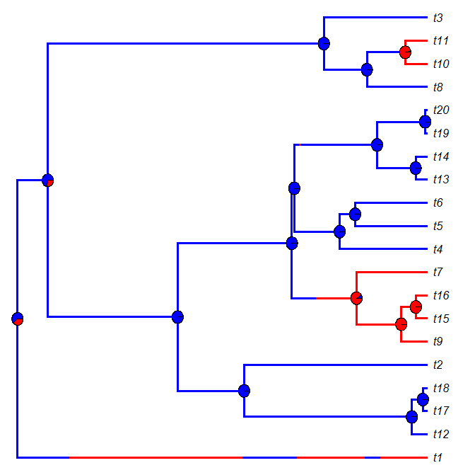
Here is the solution - by way of simulated example. Within this example, I also show how to compute the relative frequency of node states in a set of stochastic mapped trees (after all, what else would we want to plot at internal nodes):

# code to simulate a tree & data
# and to perform stochastic mapping
tree<-pbtree(n=20)
Q<-matrix(c(-1,1,1,-1),2,2)
colnames(Q)<-rownames(Q)<-c(0,1)
x<-sim.history(tree,Q,anc="0")$states
mtrees<-make.simmap(tree,x,nsim=100)
# end simulation code

# function to compute the states
foo<-function(x){
  y<-sapply(x$maps,function(x) names(x)[1])
  names(y)<-x$edge[,1]
  y<-y[as.character(length(x$tip)+1:x$Nnode)]
  return(y)
}
XX<-sapply(mtrees,foo)
pies<-t(apply(XX,1,function(x,levels,Nsim) summary(factor(x,levels))/Nsim,levels=c("0","1"),Nsim=100))
# done computing the states

# code to plot the tree
mtrees<-rescaleSimmap(mtrees,1)
cols<-c("blue","red"); names(cols)<-c(0,1)
par(mar=rep(0.1,4))
plot.phylo(mtrees[[1]],plot=FALSE,no.margin=T)
plotSimmap(mtrees[[1]],cols,pts=FALSE,lwd=3,ftype="off", add=TRUE)
text(1,1:length(mtrees[[1]]$tip),mtrees[[1]]$tip.label, pos=4,font=3)
nodelabels(pie=pies,cex=0.6,piecol=cols)
# done plotting

And here is the result of one such simulation & plotting exercise:

For fun, let's compare this to densityMap:

> densityMap(mtrees,lwd=6)
sorry - this might take a while; please be patient

Cool.