My article with Luke Mahler, Pedro Peres-Neto, and Ben Redelings just came out "Early View" (it was previously available as an accepted article in manuscript form) on the 'Evolution' journal website. Direct link here. This paper describes in detail a new Bayesian method for identifying the location of a shift in the evolutionary rate for a continuously valued trait. I have previously discussed this method in several prior blog posts that I won't list here, but that are all linked in a prior post. This is a relatively simple model for variation in the evolutionary process through time, but I am working on developing this general approach to other problems in comparative biology.
Unfortunately, the journal transposed Luke's first initials from D. Luke Mahler to Luke D. Mahler in the author list of the article copy. That this is how it will appear in print is mostly my fault as the error was in the proofs and I did not catch it. Sorry Luke!
Tuesday, September 27, 2011
Friday, September 23, 2011
New version of phytools (v0.0-9)
I just posted a new version of the "phytools" package (version 0.0-9) to my R phylogenetics page. The package is available both as Windows binary & as source. This version includes updates to the function evol.vcv() (described here) as well as:
1. phyl.cca(): a function for phylogenetic canonical correlation analysis (Revell & Harrison 2008). This function is described here & here.
2. sim.history(): a function for simulating stochastic character histories, under some model (described here).
3. sim.rates(): a function for simulating multiple evolutionary rates for a continuous character on the tree. This function is described here.
This version is not yet available on CRAN, but can be downloaded and installed from my website. Thanks for checking it out!
Simulating multiple evolutionary rates on a tree
I just created a function that will simulate multiple evolutionary rates in different parts of a phylogeny with branch lengths. The different rate regimes are specified by the user using the stochastic mapping format of make.simmap(), read.simmap(), and the new function sim.history(). It is available from my R phylogenetics page (direct link to code here) and will eventually be part of the "phytools" package.
The way this function works is incredibly simple. It essentially acts as an elaborate wrapper for my fast Brownian motion simulator, fastBM(). Basically, it creates a new "phylo" object in which the parts of each branch in each rate are scaled by the rate. This was straightforward to do from the command like with simmap format trees before. Say, for instance, we had two mapped states "blue" and "green"; and we wanted to simulate a rate of σ2=1.0 on the "blue" branches and a rate of σ2=10 on the "green" branches, we could just do the following:
> tree<-mtree
> tree$edge.length<-mtree$mapped.edge[,"blue"]*1.0+ mtree$mapped.edge[,"green"]*10
> x<-fastBM(tree)
The reason this works is because the realized outcome from a stochastic simulation on a tree (that is, the variance among species) is a function of the elapsed time (the branch length) multiplied by the evolutionary rate or instantaneous variance of the BM process on that branch. By first scaling each branch or branch segment by the desired evolutionary rate, we can then evolve by BM with a rate of σ2=1.0 on the rescaled tree to obtain the desired evolutionary rate heterogeneity.
The new function sim.rates() exploits the same principle. Let me illustrate sim.rates() with an example that also uses sim.history().
First, load "phytools" and the source files for sim.rates() and sim.history():
> require(phytools)
> source("sim.history.R")
> source("sim.rates.R")
Now, let's simulate a stochastic tree and character history using the "ape" function rbdtree() and sim.history(). We can also plot the history using plotSimmap():
> tree<-rbdtree(b=1,d=0,Tmax=log(12.5))
> Q<-matrix(c(-1,1,1,-1),2,2) # for sim.history
> mtree<-sim.history(tree,Q)
> plotSimmap(mtree)
Now, we should have something that looks like this:
Next, let's simulate on this tree using two different rates: σ2=1 on the branches and branch segments labeled "1" (and painted black in the figure above); and σ2=20 along the branches labeled "2" (red branches). If we turn the option plot to TRUE, we can even visualize the rate heterogeneity:
> rates<-c(1,20); names(rates)<-c(1,2)
> x<-sim.rates(mtree,sig2=rates,plot=T)
Finally, if we'd like to "prove" to ourselves that the data in x has indeed been generated under the intended two-rate model, we can fit the model to our tree & data using brownie.lite() (which is based on O'Meara et al. 2006):
> brownie.lite(mtree,x)
. . .
$sig2.multiple
1 2
0.7987023 22.5603855
$a.multiple
[1] 1.47557
$vcv.multiple
1 2
1 0.1720410 -0.5169118
2 -0.5169118 81.5076461
$logL.multiple
[1] -50.03446
$k2
[1] 3
$P.chisq
[1] 0.0005468257
$convergence
[1] "Optimization has converged."
(Some parts of the output from brownie.lite() have been excluded here).
Cool!
The way this function works is incredibly simple. It essentially acts as an elaborate wrapper for my fast Brownian motion simulator, fastBM(). Basically, it creates a new "phylo" object in which the parts of each branch in each rate are scaled by the rate. This was straightforward to do from the command like with simmap format trees before. Say, for instance, we had two mapped states "blue" and "green"; and we wanted to simulate a rate of σ2=1.0 on the "blue" branches and a rate of σ2=10 on the "green" branches, we could just do the following:
> tree<-mtree
> tree$edge.length<-mtree$mapped.edge[,"blue"]*1.0+ mtree$mapped.edge[,"green"]*10
> x<-fastBM(tree)
The reason this works is because the realized outcome from a stochastic simulation on a tree (that is, the variance among species) is a function of the elapsed time (the branch length) multiplied by the evolutionary rate or instantaneous variance of the BM process on that branch. By first scaling each branch or branch segment by the desired evolutionary rate, we can then evolve by BM with a rate of σ2=1.0 on the rescaled tree to obtain the desired evolutionary rate heterogeneity.
The new function sim.rates() exploits the same principle. Let me illustrate sim.rates() with an example that also uses sim.history().
First, load "phytools" and the source files for sim.rates() and sim.history():
> require(phytools)
> source("sim.history.R")
> source("sim.rates.R")
Now, let's simulate a stochastic tree and character history using the "ape" function rbdtree() and sim.history(). We can also plot the history using plotSimmap():
> tree<-rbdtree(b=1,d=0,Tmax=log(12.5))
> Q<-matrix(c(-1,1,1,-1),2,2) # for sim.history
> mtree<-sim.history(tree,Q)
> plotSimmap(mtree)
Now, we should have something that looks like this:

Next, let's simulate on this tree using two different rates: σ2=1 on the branches and branch segments labeled "1" (and painted black in the figure above); and σ2=20 along the branches labeled "2" (red branches). If we turn the option plot to TRUE, we can even visualize the rate heterogeneity:
> rates<-c(1,20); names(rates)<-c(1,2)
> x<-sim.rates(mtree,sig2=rates,plot=T)

Finally, if we'd like to "prove" to ourselves that the data in x has indeed been generated under the intended two-rate model, we can fit the model to our tree & data using brownie.lite() (which is based on O'Meara et al. 2006):
> brownie.lite(mtree,x)
. . .
$sig2.multiple
1 2
0.7987023 22.5603855
$a.multiple
[1] 1.47557
$vcv.multiple
1 2
1 0.1720410 -0.5169118
2 -0.5169118 81.5076461
$logL.multiple
[1] -50.03446
$k2
[1] 3
$P.chisq
[1] 0.0005468257
$convergence
[1] "Optimization has converged."
(Some parts of the output from brownie.lite() have been excluded here).
Cool!
Thursday, September 22, 2011
New function: sim.history()
I just posted a new function that simulates stochastic character histories for a discretely valued character trait. This function is called sim.history(), and a directly link to the source is here. The analysis is highly similar to stochastic character mapping (e.g., here), except that the simulation is unconstrained by actual data. Unlike the "geiger" function sim.char(), which can also do discrete character simulation, sim.history() simulates not only the states at the tips of the tree, but also the states at all the internal nodes of the tree as well as the timing of all the simulated transitions between states. The format for storing this information in memory is the same as used by read.simmap() (>=v0.2) and make.simmap().
To simulate, we first need our instantaneous transition matrix, Q. Let's make Q symmetric, but with uneven rates among states. For fun, let's also call our three states "blue", "green", and "red".
> source("sim.history.R")
> Q<-matrix(c(-1,0.8,0.2,0.8,-1.2,0.4,0.2,0.4,-0.6),3,3, dimnames=list(c("red","green","blue"),c("red","green","blue")))
> Q
red green blue
red -1.0 0.8 0.2
green 0.8 -1.2 0.4
blue 0.2 0.4 -0.6
Now let's get a stochastic birth-death tree:
> require(ape)
> tree<-rbdtree(birth=1.0,death=0.0,Tmax=log(25/2))
Finally, let's simulate on the tree & plot:
> mtree<-sim.history(tree,Q)
> cols<-rownames(Q); names(cols)<-rownames(Q)
> plotSimmap(mtree,cols)
And we get the following (obviously individual results will vary):
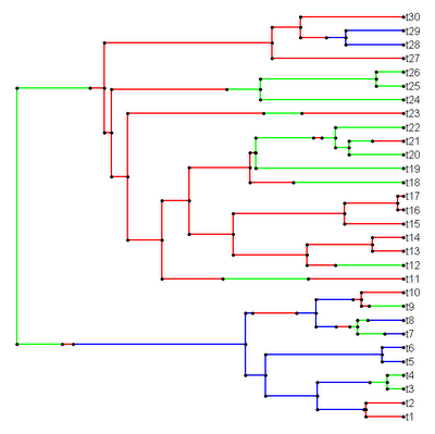
Both the node & tip states are also stored in the modified "phylo" object: here as $node.states and $states. I include this mainly to facilitate some analyses that I have been working on.
This function should be added to the next version of "phytools".
Tuesday, September 20, 2011
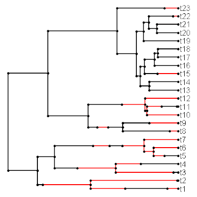
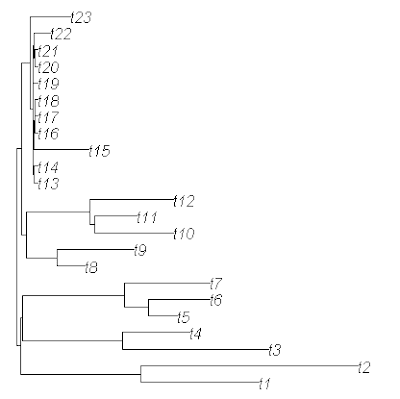
Dropping the same set of taxa from a set of trees
In response to an earlier post, a reader just inquired as to whether there was a simple way to drop the same set of terminal species from a set of trees - say a sample of trees from the posterior distribution. In fact, this can be done a couple of different ways.
A set of trees read by the "ape" functions read.tree() or read.nexus() are stored in memory as a object of class "multiPhylo". This is merely a list of objects of class "phylo" with the class "multiPhylo" assigned. First, let's generate a simple "multiPhylo" object composed of three ten-taxon trees:
> require(ape)
> trees<-list(rtree(10),rtree(10),rtree(10))
> class(trees)<-"multiPhylo"
Normally this object would be created (with class assigned) by read.tree() or read.nexus(), but for the purposes of illustration, this will do.
Next, let's say we want to prune species "t6" and "t8" from all of the trees in the list. We can do this for any individual tree using drop.tip(), e.g.:
> pruned.tree<-drop.tip(trees[[1]],c("t6","t8"))
We can prune these taxa all at once from all the trees in our set using the R "base" function lapply(). Here we would just do:
> pruned.trees<-lapply(trees,drop.tip,tip=c("t6","t8"))
> class(pruned.trees)<-"multiPhylo"
Assigning the class is necessary because lapply() returns a generic list with no class assigned. Now if we type:
> plot(pruned.trees)
we see that we have indeed pruned the desired taxa from each tree in our set. For a longer list, we can easily read the list in from a file, and then send the result object to lapply(...,drop.tip,...).
Note that this can also be done with a simple for() loop, e.g.:
> pruned.trees<-list(); class(pruned.trees)<-"multiPhylo"
> for(i in 1:length(trees))
pruned.trees[[i]]<-drop.tip(trees[[i]],c("t6","t8"))
This is more intuitive, particularly for people experienced in other programming languages like C, but will usually run slower in R.
Friday, September 9, 2011
SICB 2012 abstracts due today!
Just a quick note to remind all the procrastinators that abstracts for oral & poster presentations at the 2012 Society for Integrative & Comparative Biology (SICB) meeting are due today! A link to the SICB site is here, along with one for the 2012 meeting site (here). I just submitted my abstract & will be talking about estimating evolutionary rates for a continuous trait based on regimes representing a reconstructed discrete character. The SICB division "DSEB - Division of Systematic & Evolutionary Biology" has been newly renamed "DPCB - Division of Phylogenetics & Comparative Biology." Hopefully this will be reflected by a high turnout of phylogenetics & comparative biology at this year's meeting.
Thursday, September 8, 2011
Lambda optimization in phyl.cca()
I just added joint λ optimization to the phylogenetic canonical correlation analysis function phyl.cca(). Direct link to code is here. This nearly matches up its functionality to my "pcca" program (here & publication here). The only thing still missing is the calculation of standardized canonical coefficients and canonical coefficients. The former are analogous to standardized regression coefficients; whereas the latter are correlations (in this case, phylogenetic correlations) between the canonical variables and the original measured traits. I will hopefully add these to a future version of the function.
Just to give a quick sense of λ to the uninitiated, λ is a scaling parameter for the off-diagonals of the "coancestry matrix" (here defined as N × N matrix containing the times above the root for each pair of N species) and the among species phenotypic correlation matrix. λ and the joint estimation of λ for multiple traits is best described in a paper by Rob Freckleton & colleages (2002). It provides a very simple way to relax the strict Brownian motion assumption of most phylogenetic analyses of this nature.
To illustrate use of this function, I will give the following example of simulating with λ = 0.75 and no correlations between the Xs & the Ys. To do this, you need to install & load "phytools," "geiger," & (naturally) their dependencies.
First, let's simulate a tree & data:
> require(phytools) # load phytools
> require(geiger) # load geiger
> source("http://faculty.umb.edu/liam.revell/phytools/phyl.cca/v0.2/phyl.cca.R") # load source
> tree<-drop.tip(birthdeath.tree(b=1,d=0,taxa.stop=101),"101")
> X<-fastBM(lambdaTree(tree,lambda=0.75),nsim=4)
> Y<-fastBM(lambdaTree(tree,lambda=0.75),nsim=3)
Here, we've simulated a random Yule tree with 100 taxa along with two sets of uncorrelated random variables.
Now, let's run phylogenetic CCA with joint estimation of λ:
> result<-phyl.cca(tree,X,Y,fixed=F)
Here's our estimate of λ:
> result$lambda
[1] 0.7524329
Here's our canonical correlations & corresponding p-values:
> result$cor
[1] 0.37263858 0.17331011 0.04891746
> result$p
[1] 0.1377030 0.7930295 0.8924366
Now, let's try the analysis with fixed lambda of λ=1.0 (the default):
> result<-phyl.cca(tree,X,Y)
> result$cor
[1] 0.5571312 0.2352854 0.1519402
> result$p
[1] 2.316245e-05 2.665493e-01 3.297459e-01
And, now without the phylogeny at all (i.e., with a star tree):
> result<-phyl.cca(starTree(tree$tip.label,rep(1,100)),X,Y)
> result$cor
[1] 0.5505426 0.2995164 0.1657136
> result$p
[1] 7.276668e-06 7.216184e-02 2.664303e-01
Although this is just a single example, it gives us a little cause for consternation because both the fixed λ and non-phylogenetic analyses show significant canonical correlations, even though we didn't simulate any!
Please let me know if you give the function a try.
Wednesday, September 7, 2011
Phylogenetic canonical correlation analysis
I just posted a new function to do phylogenetic canonical correlation analysis. Canonical correlation is a procedure whereby, given two sets of variables (say, a set of Xs and a set of Y), we identify the orthogonal linear combinations of each that maximize the correlations between the sets. This type of analysis is most naturally used in an evolutionary study to analyze, say, a set of morphological variables and a set of environmental or ecological variables.
The phylogenetic version of this analysis takes the phylogeny and a (explicit or implicit) model of evolution into account to find the linear combination of Xs and Ys that maximizes the evolutionary correlations (that is, the inferred correlation of evolutionary changes) between the two sets (Revell & Harrison 2008).
The program is very simple. Direct link to the code is here. To use the function, first load the source:
> source("http://faculty.umb.edu/liam.revell/phytools/phyl.cca/v0.1/phyl.cca.R")
> result<-phyl.cca(tree,X,Y)
Here, tree is a phylogenetic tree; and X & Y are two data matrices containing values for one or multiple characters in columns and species in rows. Rows should be named by species.
The results are returned as a list with the following elements:
> result
$cor
[1] 0.3764753 0.1852836 0.1054606
$xcoef
CA1 CA2 CA3
[1,] 0.04497549 -0.09956576 -0.45926364
[2,] -0.18997199 0.46065246 -0.07810429
[3,] -0.42425815 -0.16063677 -0.18791902
[4,] 0.25374826 0.29822455 -0.06176255
$ycoef
CA1 CA2 CA3
[1,] -0.2704762 -0.3841450 0.1029158
[2,] -0.1048448 0.2502089 0.5860655
[3,] 0.3736474 -0.2580132 0.2743137
$xscores
CA1 CA2 CA3
1 0.27821077 -0.33344726 0.94985154
2 -0.23088044 0.78905936 0.26050453
3 -1.44525534 -0.22803129 -0.64071476
...
$yscores
CA1 CA2 CA3
1 0.55710619 -0.850905958 0.300282830
2 1.41482268 1.237829442 -0.446763906
3 -1.40453596 0.227361557 -0.964307876
...
$chisq
[1] 8.9531203 2.0752824 0.5032912
$p
[1] 0.7069293 0.9126462 0.7775202
Here, $cor is the set of canonical correlation; $xcoef & $ycoef are the canonical coefficients; $xscores & $yscores are the canonical scores, in terms of the original species; and $chisq & $p are Χ2 with corresponding p-values. The p-values are properly interpreted as the probability that the ith and all subsequent correlations are zero.
A few years ago I released a C program that does more or less the same thing; however there are a few differences.
1) My C program globally optimizes the λ parameter. I will add this to the present function promptly.
2) My C program first transforms the data into a phylogeny free space, and then computes the canonical correlations. This means that, although the correlations are the same in both methods, the scores are no longer in terms of species and will be different than in this function.
It is also possible to conduct a non-phylogenetic canonical correlation analysis with this function by giving phyl.cca() a star phylogeny with unit length. To do this with our previous example, we can just do the following:
> result<-phyl.cca(starTree(species=tree$tip.label, branch.lengths=rep(1,length(tree$tip))),X,Y)
This should produce the same result as cc() in the "CCA" package. (Note, though, that for cc() the rows of X & Y must be in the same order - they do not for phyl.cca(), but must contain row names.)
This function will be added to the next update of "phytools".
Thursday, September 1, 2011
Negative estimated variances from the likelihood surface
A user recently reported a problem with estimation of the variances from the likelihood surface in evol.vcv(). This is done by first computing the Hessian matrix (the matrix of partial second derivatives) of the likelihood surface at the optimum, and then calculating the negative inverse of this matrix. This matrix is the (asymptotic) variance-covariance matrix of our ML parameter estimates. The element-wise square root of the diagonal should then provide the (asymptotic) standard errors.
The user reported problem is that in some rare cases an estimated variance obtained this way is negative. Although via troubleshooting I have managed to eliminate some possible reasons for this problem (for instance, failure to converge or errors in the calculation of the Hessian), I still have not managed to figure out why this is the case. I have not eliminated the possibility that this might have something to do with reparameterizing the likelihood optimization in terms of the Cholesky matrices. [Note that I then compute the Hessian from the likelihood function in terms of the VCV matrix.] Any suggestions (e.g., Carl?) are welcome!
The user reported problem is that in some rare cases an estimated variance obtained this way is negative. Although via troubleshooting I have managed to eliminate some possible reasons for this problem (for instance, failure to converge or errors in the calculation of the Hessian), I still have not managed to figure out why this is the case. I have not eliminated the possibility that this might have something to do with reparameterizing the likelihood optimization in terms of the Cholesky matrices. [Note that I then compute the Hessian from the likelihood function in terms of the VCV matrix.] Any suggestions (e.g., Carl?) are welcome!
Subscribe to:
Posts (Atom)