New completely re-written version of phylomorphospace with mapped discrete trait

I just posted a new, completely re-written version of phylmorphospace - the phytools function that does a projection of the tree into a two dimensional morphospace. Since I wrote the original version way back in 2010, and the guts of the function had persisted largely unchanged since that time, this was probably overdue.

There was no major issue with the prior version; however I wanted to add some features and realized that the code could be a lot nicer - so I decided to re-write the function (pretty much) from scratch.

Phylomorphospace plots are pretty easy in principle. We just need to supply tip states & compute or supply all the states at internal nodes. Having done that, we can just plot all the tip & node states in our bivariate morphospace, and then add edges connecting all parent & daughter nodes.

Source code for the updated version of phylomorphospace is here; I have also posted a new build of phytools with these updates (phytools 0.2-38).

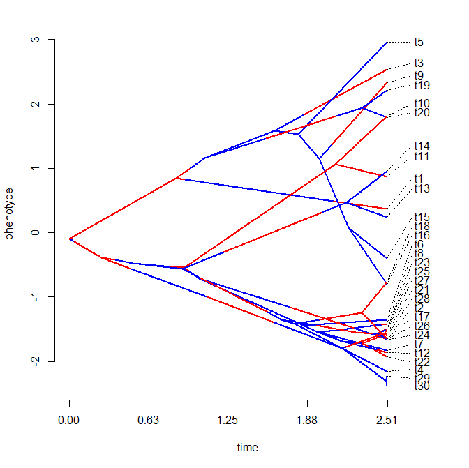
The update that inspired the re-write was that I wanted to be able to plot the state of a mapped discrete character along the edges of the tree, à la (for example) this version of phenogram. To do this for a projection of the tree into two dimensions is a little more complicated, because in phenogram the time spent in a mapped state is just plotted on the interval demarcated by the horizontal (i.e., time) axis. In two phenotypic trait dimensions, this is a little more complicated. Here, we have to compute the proportion of time spent in each state on each edge and then color the edge proportionally by those states, accordingly.

OK, here's a quick demo:

> require(phytools)
Loading required package: phytools
> packageVersion("phytools")
[1] ‘0.2.38’
> # first the standard version
> tree<-pbtree(n=20,scale=1)
> X<-fastBM(tree,nsim=2)
> phylomorphospace(tree,X,xlab="X1",ylab="X2")

OK, now for something more interesting let's simulate a discrete character on the tree; and then generate data for two continuous traits in which both the rate & evolutionary correlation differ depending on the mapped discrete character:

> Q<-0.5*matrix(c(-1,1,1,-1),2,2)
> rownames(Q)<-colnames(Q)<-letters[1:2]
> mtree<-sim.history(tree,Q,anc="a")
> # here's our discrete character history on the tree
> plotSimmap(mtree,colors=cols,pts=F)>

> # this is for simulation
> R<-list(matrix(c(0.5,0.45,0.45,0.5),2,2),
+ matrix(c(2,0,0,2),2,2))
> names(R)<-letters[1:2]
> X<-sim.corrs(mtree,R)
> cols<-c("blue","red"); names(cols)<-letters[1:2]
> phylomorphospace(mtree,X,xlab="X1",ylab="X1",colors=cols)

Pretty cool, I guess.... The evolutionary pattern that we simulated - low rate & high evolutionary correlation on the blue branches; & high rate but low evolutionary correlation on the red branches - is pretty evident in the plot.

One little note about plotting tip labels. During the re-write I noticed that I'd used the function textxy from the package 'calibrate' in place of the base graphics function text - but I'd forgotten why. Turns out textxy is a neat function that plots text labels for points with an offset that varies depending on the plot quadrant. This is perfect for a function like phylomorphospace, because it helps push the labels away from other plotted lines & points.

That's it for now.