Phylomorphospace plotting

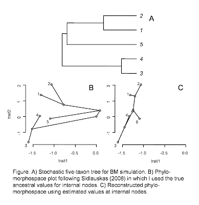
I created panels (B) and (C) of the plot at right using a new function I wrote to reproduce the so-called "phylo-morphospace" graphing method of Sidlauskas (2008). Note that this function is available without guarantees, but I would happy to hear about its success or failure on your dataset.

The function, which is available here, takes a tree and two matrices as input. The first matrix is n x 2 and contains the tip values for two traits in n species on the tree (n=5 in this case). The second matrixis m x 2 for m internal nodes and contains the values (known or estimated) for each internal node in the tree, including the root.

To create the panels, I first simulated BM evolution for two traits on the five-taxon stochastic tree in panel (A). I stored both the ancestral trait values and the tip values for terminal species (more on that later).

For panel (B) I sent my function the tip values, along with the known values for internal nodes from the simulation. For panel (C), I first estimated internal node states for the two characters using the "ape" function ace() (ancestral character estimation) under ML. This latter scenario would be more typical of empirical studies.

The contrast between (B) and (C) is pretty neat in this case. This is because in the simulation the true states at internal nodes are nearly invariably (with the exception of the MRCA of species 3 & 4) beyond the range of the observed data for the terminal species in our tree.

I will write more on programming the phylomorphospace plotting function as well as on simulating data while retaining the states at internal nodes in subsequent posts.