New postdoc in phylogeny methods

I am hiring a new postdoc in phylogenetic comparative methods. The job advertisement is below:

-----------------------------------

Postdoctoral research associate in phylogenetic comparative methods

A postdoctoral position is available in the Revell lab (http://faculty.umb.edu/liam.revell/) at the University of Massachusetts Boston in theoretical phylogenetics and/or computational phylogeny methods. Applicants should have a Ph.D. and extensive training and experience in one or more of the following areas: phylogeny method development or application in software; theoretical evolutionary quantitative genetics; and/or evolutionary computational biology. The ideal candidate will also have broad training in evolutionary biology, strong writing skills, and prior teaching or mentoring experience.

The postdoc hired from this search will play a key role in a recently funded NSF project to develop and apply new methods for evolutionary analysis in the context of phylogenetic trees. Major goals of this project include developing new visualization methods for phylogenetic comparative biology, improving the integration of phylogeny inference and comparative analysis, and bridging micro- and macroevolution in phylogenetic comparative biology. Consequently, the best candidate for this position will have skills and experience in multiple areas. The project also has substantial training goals, including the development of a new series of phylogenetic analysis mini-courses in Latin America, and a young developers’ workshop at UMass Boston’s Nantucket Field Station. The successful candidate will also be expected to participate in some of these programs.

The position is available for one year with the possibility of renewal. Start date is flexible. Please email Liam Revell (liam.revell@umb.edu) with any questions about this position.

A complete application for this position will include: (1) a brief cover letter; (2) a curriculum vitae; (3) a maximum two-page statement of your research experience & interest; and (4) names & contact information for three references. Applications can be submitted online via UMass Boston’s Interview Exchange system via the following URL: http://www.phytools.org/postdoc.search/. The position is open until filled, but applications should be sent by May 29, 2014 for full consideration.

UMass Boston provides equal employment opportunities (EEO) to all employees and applicants for employment.

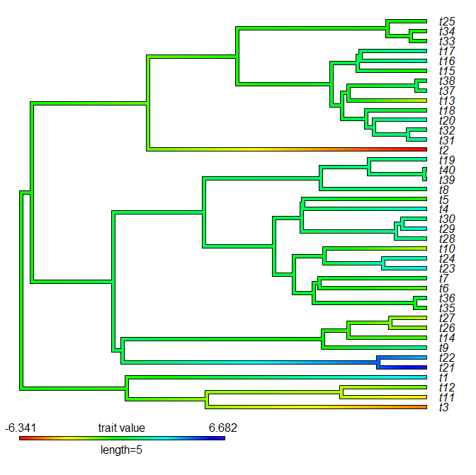
New option to offset tip labels in contMap and densityMap

In response to a recent Facebook request I just added the option to offset tip labels in the phytools functions contMap and densityMap. This is simple. Because plot.contMap and plot.densityMap (the plotting methods for objects returned by each function) use plotSimmap internally, all I had to do was migrate that option to plotSimmap. To get this functionally, users will have to update phytools to a version >=0.4-03 (e.g., here). As of writing, this is not on CRAN.

Here's a quick demo using contMap:

> require(phytools)
Loading required package: phytools
Loading required package: ape
Loading required package: maps
Loading required package: rgl
> packageVersion("phytools")
[1] ‘0.4.3’
> tree<-pbtree(n=40,scale=10)
> x<-fastBM(tree)
> obj<-contMap(tree,x)

OK, now say I'm unhappy with the spacing of my tip labels. I can now do:

> plot(obj,offset=1)

adjusting offset until satisfied. Cool.

Note that although the offset is adjusted, the x-axis limits are not. This could create a problem for a large offset, & I will fix this in future so that xlim is under user control; however, plot.contMap and plot.densityMap already allow a fairly generous space to the right of tip labels anyway.

Finally, this will not work for type="fan". This is the same as in plotSimmap, so addressing this will take a little more effort than I'm willing to invest at this precise moment in time.

New print & plot methods for describe.simmap

I just added new print & plot methods to phytools for the object returned by describe.simmap, a function designed to summarize the results of stochastic mapping conducted with the phytools function make.simmap. Here's a quick demo:

> require(phytools)
Loading required package: phytools
Loading required package: ape
Loading required package: maps
Loading required package: rgl
> packageVersion("phytools")
[1] ‘0.4.2’
> data(anoletree)
> x<-getStates(anoletree,"tips")
> trees<-make.simmap(anoletree,x,nsim=100,model="ER",
  message=FALSE)
> obj<-describe.simmap(trees)
> ## print method
> obj
100 trees with a mapped discrete character with states:
 CG, GB, TC, TG, Tr, Tw

trees have 25.88 changes between states on average

changes are of the following types:
     CG,GB CG,TC CG,TG CG,Tr CG,Tw GB,CG GB,TC GB,TG GB,Tr
x->y  0.27  0.39  0.29  0.18  0.37  0.53  0.77  0.96  0.39
     GB,Tw TC,CG TC,GB TC,TG TC,Tr TC,Tw TG,CG TG,GB TG,TC
x->y  1.09  1.23  0.74  0.51  0.71  0.94  1.15  3.32  1.89
     TG,Tr TG,Tw Tr,CG Tr,GB Tr,TC Tr,TG Tr,Tw Tw,CG Tw,GB
x->y  1.05  1.78  0.21  0.29  0.21  0.21  0.28  0.86   1.8
     Tw,TC Tw,TG Tw,Tr
x->y  1.82  0.97  0.67

mean total time spent in each state is:
             CG         GB         TC        TG          Tr
raw  12.9528230 44.2907143 32.4717543 69.734876 12.85247436
prop  0.0629796  0.2153516  0.1578851  0.339067  0.06249168
            Tw   total
raw  33.364318 205.667
prop  0.162225   1.000

> ## plot method
> plot(obj,fsize=0.6,cex=c(0.6,0.3),ftype="i")
> ## add legend
> states<-sort(unique(getStates(trees[[1]],"tips")))
> add.simmap.legend(colors=
  setNames(palette()[1:length(states)],states),fsize=0.8)
Click where you want to draw the legend

That's not bad. The plotted pies at nodes (and tips) give the posterior probability of each node being in each state from (in this case) empirical Bayesian stochastic character mapping.

The code for these new methods, and the updated describe.simmap, is here; and a new phytools build with these methods can be downloaded from the phytools page.

Computing the height above the root of a node in the tree

phytools already has a function that computes the height of all the nodes in the tree: nodHeights. If we only want to know the height of one node, then using this function is very inefficient, for obvious reasons.

The following is alternative code for computing the height of only one node. It uses the phytools internal function getAncestors, so if we are not using it as part of phytools we will first have to do:

getAncestors<-phytools:::getAncestors

And here is the function:

nodeheight<-function(tree,node){
  if(node==(length(tree$tip.label)+1)) h<-0
  else {
    a<-setdiff(c(getAncestors(tree,node),node),
      length(tree$tip.label)+1)
    h<-sum(tree$edge.length[sapply(a,function(x,e)
      which(e==x),e=tree$edge[,2])])
  }
  h
}

That's it.

New options & methods for ltt95

A couple of days ago I received the following comment about the phytools function ltt95:

"I'm using ltt95 function with the times method and log transformed y axis, but I get reversed ages (both in the plot and in the results table). I’ve not been able to tackle down this small issue."

Well, this isn't precisely a bug of ltt95. ltt95 merely records the accumulation of lineages forward in time from the root; rather than backward (as I believe is more common in publications) from the present time.

In a newly updated version of the function I have now added the argument xaxis which can assume three values: "standard" (forward in time lineage accumulation, as in the current CRAN version of phytools); "flipped" (the time-from-the-present plot); and "negative" (similar to "flipped", but with negative time from the present). At the same time I also have modified ltt95 to return an object of class "ltt95" invisibly (don't worry, this is just the same matrix with some attributes); and I have added S3 generic plotting & print methods for objects of this class.

Here's a demo - but the function can be used in more diverse ways than I will demonstrate here:

> library(phytools)
Loading required package: ape
Loading required package: maps
Loading required package: rgl
> packageVersion("phytools")
[1] ‘0.4.0’
> ## simulate some trees
> trees<-pbtree(n=100,scale=50,nsim=100)
> trees
100 phylogenetic trees
> ## run ltt95
> obj<-ltt95(trees)

> ## ok, now let's flip the axis & plot on semi-log
> ## (I could have done this originally too)
> obj
Object of class "ltt95".
  alpha:        0.05
  method:       lineages
  mode:         median
  N(lineages):  100
> plot(obj,xaxis="flipped",log=TRUE)

Code for this new function version is here and it is in a phytools build, which can be downloaded & installed from source.

That's all for now.

New function to paint individual branch or branches of the tree

A few days ago I received the following email:

"I have recently come across your excellent paper entitled "On the analysis of evolutionary change along single branches in a phylogeny". In that you employed a software "available on request", so I am writing to request permission to obtain and use your software. Alternatively, I wonder whether the functions from that software were incorporated into the Phytools R package. I am sorry if I am missing the obvious and it is indeed in the Phytools package - I am not familiar with all functions in that package yet."

(One interesting attribute of this message is that it harks back to a day in the not too distant past in which sharing data or software 'on request' seemed more than reasonable - how quaint & passé that seems today!)

The paper that's being referred to here is Revell (2008; Am. Nat.) in which I show that a (at that time) new likelihood method by O'Meara et al. (2006) could be used to test hypotheses about exceptional evolution along (one or more) single branch(es) of the tree. Previously McPeek (1995) had proposed a cruder approach based loosely on contrasts, which I showed had reasonable type I error; however I also showed that the likelihood method was probably preferable under most circumstances.

Indeed this method is available in phytools in the form of brownie.lite; although to 'paint' branches which we have a priori hypothesized to have a higher or lower evolutionary rate is a little bit tricky. I decided to make this a whole lot easier by adding the function paintBranches to the phytools package (new source build here).

Here is an example workflow using the function to test the hypothesis of a higher rate of evolution along a specific branch of the tree:

> library(phytools)
Loading required package: ape
Loading required package: maps
Loading required package: rgl
> packageVersion("phytools")
[1] ‘0.3.99’
> ## simulate data with a high rate on one branch
> tree<-pbtree(n=26,tip.label=LETTERS[26:1])
> plotTree(tree)
> nodelabels()

> ## stretch one of the branches by x 100
> tt<-tree
> tt$edge.length[which(tt$edge[,2]==29)]<-
 tt$edge.length[which(tt$edge[,2]==29)]*100
> ## simulate data on distorted tree
> x<-fastBM(tt)
> ## paint branch with second regime to fit 2-rate model
> tree<-paintBranches(tree,29,"2")
> plotSimmap(tree,lwd=4)
no colors provided. using the following legend:
      1       2
"black"   "red"
> nodelabels()

> fit<-brownie.lite(tree,x)
> fit
ML single-rate model:
        s^2     se      a       k  logL
value   1.41    0.39    1.35    2  -39.37 

ML multi-rate model:
        s^2(1)  se(1)   s^2(2)  se(2)   a       k  logL 
value   0.96    0.26    40.24   60.27   0.12    3  -35.82

P-value (based on X^2): 0.01

R thinks it has found the ML solution.

We can use the same approach if our hypothesized exceptional regime is found on several branches in the tree. In this case, the function argument edge is an integer vector instead of a single node number. Finally, if we have an a priori hypothesis of multiple classes of exceptional rate, we can test that too using multiple calls to paintBranches.

That's it.