Dave Bapst kindly pointed out that the function anc.ML() will fail if there are any zero length internal or terminal branches in the tree.
For zero length tip edges this is unavoidable because the determinant of vcvPhylo(tree) for this tree will always be zero. However, for zero length internal edges this can be avoided by first collapsing these using the ape function di2multi(). Unfortunately, anc.ML could not handle these trees because it uses pic() to estimate a starting value for the evolutionary rate, σ2!
Fortunately, I have resolved this by way of a couple of fixes. 1) The function first checks if the tree contains any zero length edges. If it does, then anc.ML will return an informative error message. 2) If the tree does contain polytomies, then pic() will be called on an arbitrarily resolved tree (using multi2di). The new version of this function is available here.
Thursday, December 8, 2011

Wednesday, December 7, 2011
Dropping a random tip (or set of tips) from a tree
In a couple of recent posts (1,2) I have commented on Google search strings that (as the administrator of this blog) I can see have led users to my site. Today, a user ended up visiting the blog due to the following search string:
"randomly drop.tip in r"
by which I take it to mean they'd like to drop a random tip (or set of tips) from a "phylo" object in R.
Here's how to do it. To drop a single tip at random just type:
tr2<-drop.tip(tr1,tr1$tip.label[ceiling(runif(n=1, max=length(tr1$tip)))])
To drop a set of tips, say m=10 random tips, just type:
tr2<-drop.tip(tr1,sample(tr1$tip.label)[1:m])
(actually, this will also work for a single tip, you just need to set m=1). Of course, if you wanted to, say, drop 30% of the taxa at random, you would just have to first compute the number of taxa to drop, m, and then apply the code above. For instance:
m<-round(0.3*length(tr1$tip))
tr2<-drop.tip(tr1,sample(tr1$tip.label)[1:m])
It's that easy!
"randomly drop.tip in r"
by which I take it to mean they'd like to drop a random tip (or set of tips) from a "phylo" object in R.
Here's how to do it. To drop a single tip at random just type:
tr2<-drop.tip(tr1,tr1$tip.label[ceiling(runif(n=1, max=length(tr1$tip)))])
To drop a set of tips, say m=10 random tips, just type:
tr2<-drop.tip(tr1,sample(tr1$tip.label)[1:m])
(actually, this will also work for a single tip, you just need to set m=1). Of course, if you wanted to, say, drop 30% of the taxa at random, you would just have to first compute the number of taxa to drop, m, and then apply the code above. For instance:
m<-round(0.3*length(tr1$tip))
tr2<-drop.tip(tr1,sample(tr1$tip.label)[1:m])
It's that easy!
Ancestral state estimation when the rate of evolution varies throughout the tree
A user contacting me recently about performing ancestral state estimation when the rate of evolution varies on the different branches of the tree. (Actually, she contacted me about another, slightly more complex problem - but this is where I'm starting.) To see why this might be an issue, consider the following tree:
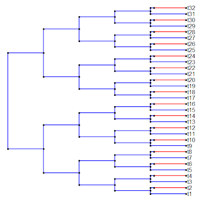
and imagine that the rate of evolution is very low [say σ(blue)2=0.01] on the blue branches of the tree, and very high [say σ(red)2=1.0] on the red branches. Under this scenario, the states at the internal nodes of the tree will be much closer in value to the state at the root node than they will be (on average) to any red tip. We might like to take this into consideration in estimating ancestral character values.
To show this, let's consider the following example. First, let's simulate data on the tree by first stretching the branches of the tree by their rates of evolution, then by using fastBM(). Here I use fastBM() rather than the much easier phytools function sim.rates(), because fastBM() allows us to return the states at internal nodes. Then, I will use anc.ML() to estimate internal node states using likelihood, ignoring heterogeneity in the evolutionary rate, and compare these estimates to the "true," normally unknown, ancestral character values.
> require(phytools)
> source("anc.ML.R")
> tree<-read.simmap(text="(((((t1:{1,1},t2:{1,0.1:2,0.9}):{1,1}...;",rev.order=F)
> cols<-c("blue","red"); names(cols)<-c(1,2)
> sig2<-c(0.01,1); names(sig2)<-c(1,2)
> simtree<-tree; simtree$edge.length<-colSums(t(tree$mapped.edge)*sig2)
> x<-fastBM(simtree,internal=T) # parts of Newick style tree not shown
> ace1<-anc.ML(tree,x[1:32])
> mse1<-mean((x[33:length(x)]-ace1$ace)^2)
> mse1
[1] 0.09184913
> plot(x[33:length(x)],ace1$ace)
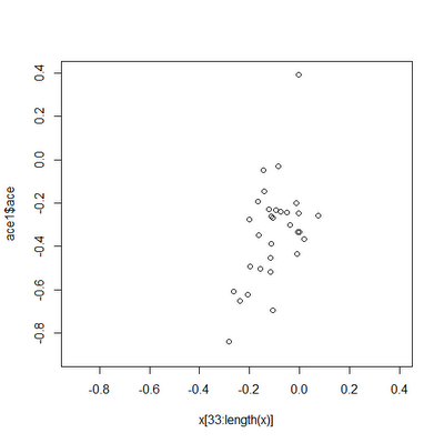
Obviously, these estimates are not great, and the ancestral state estimates (on the y-axis) span a much broader range than the true values, as we might expect. [I have plotted the points on a square set of axes just to make this point clear.] Now, for comparison, let's first fit a multi-rate BM model and then try to use the fitted rates to inform our ancestral character estimation on the tree:
> fit<-brownie.lite(tree,x[1:32])
> fit
...
$sig2.multiple
1 2
0.005546321 0.684734146
...
$P.chisq
[1] 2.143502e-11
> fittree<-tree
> fittree$edge.length<- colSums(t(tree$mapped.edge)*fit$sig2.multiple)
> ace2<-anc.ML(fittree,x[1:32])
> mse2<-mean((x[33:length(x)]-ace2$ace)^2)
> mse2
[1] 0.005524579
> plot(x[33:length(x)],ace2$ace)
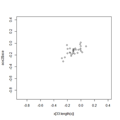
Clearly, the estimates are much closer to the true values in this case.
To be perfectly transparent, this particular example is designed to be an extreme case, and for most trees & datasets, the effect will be much smaller.

and imagine that the rate of evolution is very low [say σ(blue)2=0.01] on the blue branches of the tree, and very high [say σ(red)2=1.0] on the red branches. Under this scenario, the states at the internal nodes of the tree will be much closer in value to the state at the root node than they will be (on average) to any red tip. We might like to take this into consideration in estimating ancestral character values.
To show this, let's consider the following example. First, let's simulate data on the tree by first stretching the branches of the tree by their rates of evolution, then by using fastBM(). Here I use fastBM() rather than the much easier phytools function sim.rates(), because fastBM() allows us to return the states at internal nodes. Then, I will use anc.ML() to estimate internal node states using likelihood, ignoring heterogeneity in the evolutionary rate, and compare these estimates to the "true," normally unknown, ancestral character values.
> require(phytools)
> source("anc.ML.R")
> tree<-read.simmap(text="(((((t1:{1,1},t2:{1,0.1:2,0.9}):{1,1}...;",rev.order=F)
> cols<-c("blue","red"); names(cols)<-c(1,2)
> sig2<-c(0.01,1); names(sig2)<-c(1,2)
> simtree<-tree; simtree$edge.length<-colSums(t(tree$mapped.edge)*sig2)
> x<-fastBM(simtree,internal=T) # parts of Newick style tree not shown
> ace1<-anc.ML(tree,x[1:32])
> mse1<-mean((x[33:length(x)]-ace1$ace)^2)
> mse1
[1] 0.09184913
> plot(x[33:length(x)],ace1$ace)

Obviously, these estimates are not great, and the ancestral state estimates (on the y-axis) span a much broader range than the true values, as we might expect. [I have plotted the points on a square set of axes just to make this point clear.] Now, for comparison, let's first fit a multi-rate BM model and then try to use the fitted rates to inform our ancestral character estimation on the tree:
> fit<-brownie.lite(tree,x[1:32])
> fit
...
$sig2.multiple
1 2
0.005546321 0.684734146
...
$P.chisq
[1] 2.143502e-11
> fittree<-tree
> fittree$edge.length<- colSums(t(tree$mapped.edge)*fit$sig2.multiple)
> ace2<-anc.ML(fittree,x[1:32])
> mse2<-mean((x[33:length(x)]-ace2$ace)^2)
> mse2
[1] 0.005524579
> plot(x[33:length(x)],ace2$ace)

Clearly, the estimates are much closer to the true values in this case.
To be perfectly transparent, this particular example is designed to be an extreme case, and for most trees & datasets, the effect will be much smaller.
Tuesday, December 6, 2011
Ancestral character estimation using likelihood
I just posted a new function for ancestral character estimation using likelihood called anc.ML(). (Direct link to code here.) This function is a lightweight version of ace() from the ape package, in that it only does likelihood estimation and only for continuously valued character traits. I developed this because I have been having trouble with ace(...,method="ML") in terms of accuracy. In particular, with some regularity (maybe 5% of the time on stochastic 100 taxon trees), the ML optimization in ace() seems to converge to the wrong ancestral character values.
One difficulty that I encountered when trying to evaluate the performance of anc.ML() was the discovery that the likelihoods reported by both functions are different. In particular, I realized that the likelihoods reported by ace() exclude constant terms. For a Brownian model, the constant terms for a set of ancestral states and rate for the BM process are two: –(n+m-1)log(2π)/2 (for n species and m internal nodes), and log(|C|)/2 (for cophenetic matrix C). Sure enough, this is exactly the amount by which the log-likelihoods returned by ace(...,method="ML") and anc.ML() differ.
First, an example when ace() is working:
> require(phytools) # needs phytools 0.1-2
> source("anc.ML.R") # load the source code for anc.ML
> set.seed(1)
> tree<-rtree(100)
> x<-fastBM(tree)
> res1<-ace(x,tree,method="ML")
> res1$loglik
[1] -29.04148
> res2<-anc.ML(tree,x,maxit=4000)
> res2$logLik
[1] -116.1555
> plot(res1$ace,res2$ace)
> res1$loglik-(length(tree$tip)+tree$Nnode-1)*log(2*pi)/2-as.numeric(determinant(vcvPhylo(tree),logarithm=T)$modulus)/2
[1] -116.1555
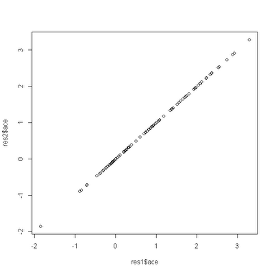
This just shows that ace(...,method="ML") and anc.ML() produce the same estimates (to a fairly high degree of precision); and that the likelihoods differ by a constant for a given tree. That is, of course, when ace() behaves. Sometimes it doesn't. Try this example:
> set.seed(90)
> tree<-rtree(100)
> x<-fastBM(tree)
> res1<-ace(x,tree,method="ML")
> res1$loglik-(length(tree$tip)+tree$Nnode-1)*log(2*pi)/2-as.numeric(determinant(vcvPhylo(tree),logarith=T)$modulus)/2
[1] -92.44219
> res2<-anc.ML(tree,x,maxit=4000)
> res2$logLik
[1] -84.40321
> plot(res1$ace,res2$ace)
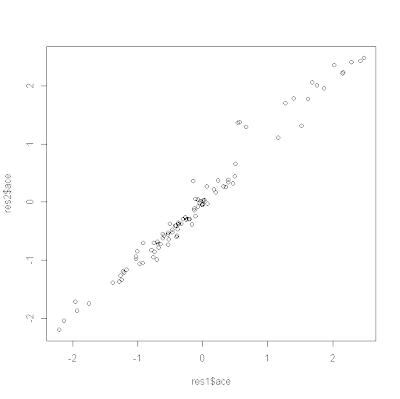
Obviously, something is amiss in this example. I was working on this to show how to do ancestral state estimation for a continuous trait when rates of evolution differ in different parts of the tree, and I will try to iron out any bugs in anc.ML as I work on this.
One difficulty that I encountered when trying to evaluate the performance of anc.ML() was the discovery that the likelihoods reported by both functions are different. In particular, I realized that the likelihoods reported by ace() exclude constant terms. For a Brownian model, the constant terms for a set of ancestral states and rate for the BM process are two: –(n+m-1)log(2π)/2 (for n species and m internal nodes), and log(|C|)/2 (for cophenetic matrix C). Sure enough, this is exactly the amount by which the log-likelihoods returned by ace(...,method="ML") and anc.ML() differ.
First, an example when ace() is working:
> require(phytools) # needs phytools 0.1-2
> source("anc.ML.R") # load the source code for anc.ML
> set.seed(1)
> tree<-rtree(100)
> x<-fastBM(tree)
> res1<-ace(x,tree,method="ML")
> res1$loglik
[1] -29.04148
> res2<-anc.ML(tree,x,maxit=4000)
> res2$logLik
[1] -116.1555
> plot(res1$ace,res2$ace)
> res1$loglik-(length(tree$tip)+tree$Nnode-1)*log(2*pi)/2-as.numeric(determinant(vcvPhylo(tree),logarithm=T)$modulus)/2
[1] -116.1555

This just shows that ace(...,method="ML") and anc.ML() produce the same estimates (to a fairly high degree of precision); and that the likelihoods differ by a constant for a given tree. That is, of course, when ace() behaves. Sometimes it doesn't. Try this example:
> set.seed(90)
> tree<-rtree(100)
> x<-fastBM(tree)
> res1<-ace(x,tree,method="ML")
> res1$loglik-(length(tree$tip)+tree$Nnode-1)*log(2*pi)/2-as.numeric(determinant(vcvPhylo(tree),logarith=T)$modulus)/2
[1] -92.44219
> res2<-anc.ML(tree,x,maxit=4000)
> res2$logLik
[1] -84.40321
> plot(res1$ace,res2$ace)

Obviously, something is amiss in this example. I was working on this to show how to do ancestral state estimation for a continuous trait when rates of evolution differ in different parts of the tree, and I will try to iron out any bugs in anc.ML as I work on this.
Saturday, December 3, 2011
Dropping the same tip from many trees in a "multiPhylo" object
Following the same theme as an earlier post, I thought I would take a closer look a Google search strings that have led readers to my site. A recent search string that has multiple hits is the following: "drop.tip multiphylo", by which I presume they mean to ask how one drops the same tip (or set of tips) from a set of phylogenies in an object of class "multiPhylo". It turns out that we can do this very easily, in fact.
First, let's get a set of trees as an object of the class "multiPhylo". [In most cases, of course, these would probably be trees we have read in from file (say, as a posterior sample of trees in a Bayesian analysis). In this case, we will just use the ape function rmtree().]
> require(ape)
> trees<-rmtree(N=10,n=20)
> trees
10 phylogenetic trees
> require(phytools)
> plotTree(trees[[6]]) # for instance
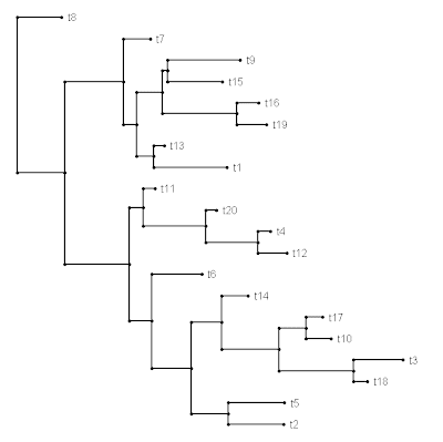
This gives a set of 10 trees, each containing 20 taxa, with the tip labels "t1" to "t20".
Now, a "multiPhylo" object is really just a list of trees, so to apply the ape function drop.tip to all the trees in the list, we can just use the function lapply. Let's drop, say "t13" (for luck) from all the trees in the list:
> ntrees<-lapply(trees,drop.tip,tip="t13")
> class(trees)<-"multiPhylo"
> plotTree(ntrees[[6]]) # for comparison
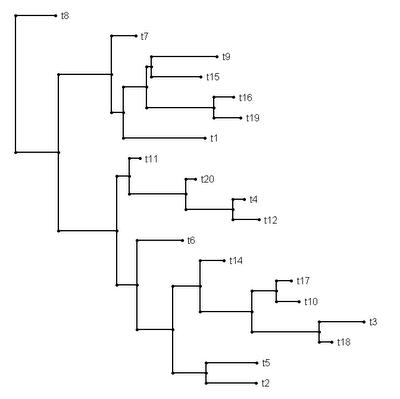
and taxon "t13" is gone, just as we'd hope. (The same is true, of course, of all the trees in our set.)
Naturally, the same technique works for a set of tips, for instance:
> ntrees<-lapply(trees,drop.tip,tip=c("t11","t12","t13"))
> class(ntrees)<-"multiPhylo"
We can even combine this with the trick, described in an earlier post that allows us to drop all but the set of taxa we have in a list. In this case, we will make the special function keep.tip. For instance if we wanted to keep only "t1" through "t10" in each of our trees above, we could just do the following:
> species<-paste("t",1:10,sep="")
> species
[1] "t1" "t2" "t3" "t4" "t5" "t6" "t7" "t8" "t9" "t10"
> keep.tip<-function(tree,tip) drop.tip(tree,setdiff(tree$tip.label,tip))
> ntrees<-lapply(trees,keep.tip,tip=species)
> "multiPhylo"->class(ntrees)
> plotTree(ntrees[[6]])
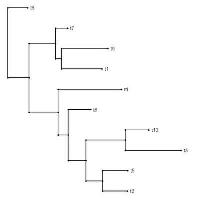
[Thanks to Dan Rabosky for the setdiff() suggestion.] Cool.
First, let's get a set of trees as an object of the class "multiPhylo". [In most cases, of course, these would probably be trees we have read in from file (say, as a posterior sample of trees in a Bayesian analysis). In this case, we will just use the ape function rmtree().]
> require(ape)
> trees<-rmtree(N=10,n=20)
> trees
10 phylogenetic trees
> require(phytools)
> plotTree(trees[[6]]) # for instance

This gives a set of 10 trees, each containing 20 taxa, with the tip labels "t1" to "t20".
Now, a "multiPhylo" object is really just a list of trees, so to apply the ape function drop.tip to all the trees in the list, we can just use the function lapply. Let's drop, say "t13" (for luck) from all the trees in the list:
> ntrees<-lapply(trees,drop.tip,tip="t13")
> class(trees)<-"multiPhylo"
> plotTree(ntrees[[6]]) # for comparison

and taxon "t13" is gone, just as we'd hope. (The same is true, of course, of all the trees in our set.)
Naturally, the same technique works for a set of tips, for instance:
> ntrees<-lapply(trees,drop.tip,tip=c("t11","t12","t13"))
> class(ntrees)<-"multiPhylo"
We can even combine this with the trick, described in an earlier post that allows us to drop all but the set of taxa we have in a list. In this case, we will make the special function keep.tip. For instance if we wanted to keep only "t1" through "t10" in each of our trees above, we could just do the following:
> species<-paste("t",1:10,sep="")
> species
[1] "t1" "t2" "t3" "t4" "t5" "t6" "t7" "t8" "t9" "t10"
> keep.tip<-function(tree,tip) drop.tip(tree,setdiff(tree$tip.label,tip))
> ntrees<-lapply(trees,keep.tip,tip=species)
> "multiPhylo"->class(ntrees)
> plotTree(ntrees[[6]])

[Thanks to Dan Rabosky for the setdiff() suggestion.] Cool.
Thursday, December 1, 2011
Testing for phylogenetic signal (K) different than 1.0
I can see as administrator of this blog some of the google search terms that lead users to the site. Today, someone ending up on the phytools blog with the following search: "phylogenetic signal k significantly different than one."
Testing for whether K (Blomberg et al. 2003) is significantly different from 1.0 is not explicitly implemented in my function phylosig(), but it is straightforward to imagine how one would go about doing it with simulation.
First, let's simulate data with strong phylogenetic signal (expected K of 1.0):
> require(phytools)
> tree<-rtree(100)
> x<-fastBM(tree)
> K<-phylosig(tree,x)
> K
[1] 1.103667
Now, let's get a null distribution for K=1.0 via simulation on our phylogeny:
> nullK<-apply(fastBM(tree,n=1000,sig2=mean(pic(x,tree)^2)),2, phylosig,tree=tree)
Finally, let's count the number of simulated K values that are more extreme than our observed value for K. I would suggest that we do this by counting the number of times that the absolute value of the logarithm of our observed value for K is no smaller than the absolute values of our simulated values for K. This just makes K=1.5 & K=0.6667 equivalent departures from BM. I.e.,
> P<-mean(abs(log(c(K,nullK)))>=abs(log(K)))
> P
[1] 0.8011988
Ok, now let's contrast this with data generated with no signal.
> x<-rnorm(n=length(tree$tip)); names(x)<-tree$tip.label
> K<-phylosig(tree,x)
> K
[1] 0.1998674
> nullK<-apply(fastBM(tree,n=1000,sig2=mean(pic(x,tree)^2)),2, phylosig,tree=tree)
> P<-mean(abs(log(c(K,nullK)))>abs(log(K)))
> P
[1] 0.000999001
Makes sense.
Testing for whether K (Blomberg et al. 2003) is significantly different from 1.0 is not explicitly implemented in my function phylosig(), but it is straightforward to imagine how one would go about doing it with simulation.
First, let's simulate data with strong phylogenetic signal (expected K of 1.0):
> require(phytools)
> tree<-rtree(100)
> x<-fastBM(tree)
> K<-phylosig(tree,x)
> K
[1] 1.103667
Now, let's get a null distribution for K=1.0 via simulation on our phylogeny:
> nullK<-apply(fastBM(tree,n=1000,sig2=mean(pic(x,tree)^2)),2, phylosig,tree=tree)
Finally, let's count the number of simulated K values that are more extreme than our observed value for K. I would suggest that we do this by counting the number of times that the absolute value of the logarithm of our observed value for K is no smaller than the absolute values of our simulated values for K. This just makes K=1.5 & K=0.6667 equivalent departures from BM. I.e.,
> P<-mean(abs(log(c(K,nullK)))>=abs(log(K)))
> P
[1] 0.8011988
Ok, now let's contrast this with data generated with no signal.
> x<-rnorm(n=length(tree$tip)); names(x)<-tree$tip.label
> K<-phylosig(tree,x)
> K
[1] 0.1998674
> nullK<-apply(fastBM(tree,n=1000,sig2=mean(pic(x,tree)^2)),2, phylosig,tree=tree)
> P<-mean(abs(log(c(K,nullK)))>abs(log(K)))
> P
[1] 0.000999001
Makes sense.
Percent variance from phyl.pca()
A user just emailed me to find out how to get the "percent variance explained" by each eigenvector from phytools' phylogenetic PCA (phyl.pca function. This is easy, just do the following:
> require(phytools)
> res<-phyl.pca(tree,X)
> diag(res$Eval)/sum(res$Eval)*100
PC1 PC2 PC3 PC4 PC5
26.83767 23.78144 20.18687 15.85040 13.34361
Cool.
> require(phytools)
> res<-phyl.pca(tree,X)
> diag(res$Eval)/sum(res$Eval)*100
PC1 PC2 PC3 PC4 PC5
26.83767 23.78144 20.18687 15.85040 13.34361
Cool.
Subscribe to:
Posts (Atom)