Saturday, November 10, 2012

Code for contMap & new minor phytools version

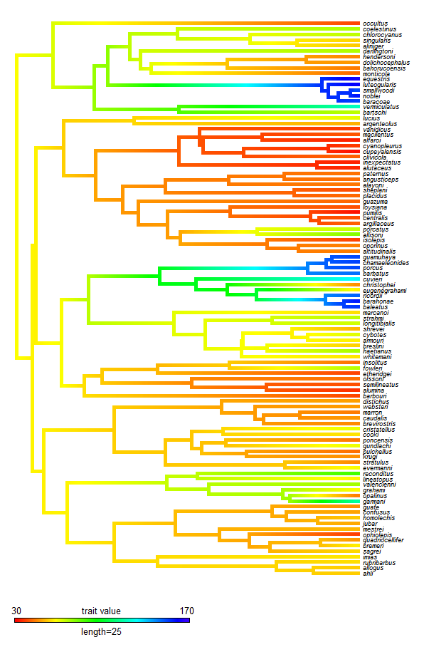
I just posted the code for contMap, a new phytools graphing function for plotting the reconstructed value of a continuous character along ancestral branches and nodes in the tree (previously described here). I made a couple of updates to the function, including some changes that allow the user to specify the trait range of the legend (previously the default was just the range of extant phenotypes). I have also built a new minor (i.e., non-CRAN) version of phytools, v0.2-05, which can be downloaded here and installed from source. Note that I have a submitted manuscript describing this function and densityMap (1, 2). See help(contMap) for citation information.

Here's a quick demo, including installation from source, again, with the Greater Antillean Anolis tree and data for SVL (data & tree not included):

> install.packages("phytools_0.2-05.tar.gz",type="source", repos=NULL)
* installing *source* package 'phytools' ...
...
* DONE (phytools)
> library(phytools)
Loading required package: ape
...
> contMap(anoletree,svl,res=200,fsize=c(0.6,0.8),outline=F, lims=c(30,170),lwd=5)
**Note, the difference between this figure and a prior iteration is because trait values are on mm rather than log(mm) scale; and I have rescaled the total tree length to 50 Ma - based on a very approximate age for the root of Greater Antillean anoles of 50 mybp (and following Mahler et al. In review).

Thursday, November 8, 2012

Mapping the reconstructed value of a quantitative character on the tree

Following my new function, densityMap, for mapping the posterior density for a discrete character from stochastic mapping on three tree (1, 2), it seemed natural to do a quantitative trait version. In this case, we just compute the ML ancestral character states at the nodes under some model (say, BM); fraction the ends into many small pieces; interpolate the states along all the edges; and then map the ancestral states to a color scheme. Note that I am interpolating using equation (3) from Felsenstein (1985), which I believe will give me the correct set of internal states. I have programmed this in a new function, contMap (continuous trait mapping), which I will soon post to the phytools page.

Here's a quick demo:
> library(phytools)
> source("contMap.R")
> tree<-pbtree(n=30)
> x<-fastBM(tree)
> contMap(tree,x,lwd=6,res=200,legend=1.5)
Pretty cool.

We can also try a "real" example. Here is body size (log SVL) in Greater Antillean anoles:
> contMap(anoletree,svl,fsize=c(0.7,1))

Trick to capitalize genus names in a phylogeny

Here's the situation: we have a tree in file or memory in which the genus names of our species binomials are not capitalized. In other words:

> plotTree(tree,ftype="i")

We want a nice plot of this tree, with minimal post hoc editing, but we need the genus names to be capitalized. Here's how to do it:

foo<-function(x){
   x<-strsplit(x,split="")[[1]]
   x[1]<-toupper(x[1])
   x<-paste(x,collapse="")
}
tree$tip.label<-sapply(tree$tip.label,foo,USE.NAMES=FALSE)
plotTree(tree,ftype="i")
That's it.

BTW: I couldn't help but notice that this is my 300th post to the phytools blog! Thanks for reading.

Monday, November 5, 2012

Update to densityMap, new minor phytools version

I just posted a new version of the function to plot the posterior density of a binary character mapped on the tree using stochastic character mapping (described here). The updated code is on the webpage for phytools, but if you want to use this function version, you are probably better off updating to the most recent, minor release of phytools, v0.2-04, here. This is because I also had to make some changes to the phytools functions plotTree, plotSimmap, and densityMap, so doing a package update from source is the best way to ensure that you have the correct versions of each function installed.

The biggest difference between this version of densityMap and the previous one is that in this version more control of how the plot looks has been migrated to the user. In particular, the user can control the width of plotted edges as well as whether or not to display a fine black outline around the lines of the tree graph. These may seem like minor changes, but to plot the outline I first use plotTree to plot a tree with lwd+2 width edges. Then I overlay the densityMap tree. To do this, I had to modify plotTree (which is actually just a wrapper for plotSimmap) so that it could be used to plot multiple trees in the same plotting object. In addition, in previous versions of plotSimmap, the offset of tip labels is a function of the plotted edge widths. This meant that when I plotted to trees in the same object, but with different width edges, the tip labels did not overlay exactly. The way I fixed this is by migrating control of the label offset to the function arguments - and then I used a label offset based only on the interior, densityMap line widths.

Here's an example of the result:
> # install package
> install.packages("phytools_0.2-04.tar.gz",type="source", repos=NULL)
** installing *source* package 'phytools' ...
...
* DONE (phytools)
> library(phytools)
Loading required package: ape
Loading required package: mnormt
...
> # simulate random Yule tree
> tree<-pbtree(n=50,scale=2)
> # simulate data on the tree using sim.history
> Q<-matrix(c(-2,2,2,-2),2,2,dimnames=list(c(0,1),c(0,1)))
> tree<-sim.history(tree,Q)
> # generating stochastic map trees (500, in this case)
> trees<-make.simmap(tree,tree$states,nsim=500)
> # create density map
> densityMap(trees,fsize=c(1,1),outline=TRUE,lwd=6, res=1000)
sorry - this might take a while; please be patient
>

Note that this is pretty slow - to make it quicker, use fewer maps (say 100) or a lower "resolution" (densityMap argument res), which is just the number of times the probability/color is sampled along any path from the root to the tips.
Friday, November 2, 2012

New minor version of phytools v0.2-03

I just posted a new minor version of 'phytools' (v0.2-03). This package version has the new function densityMap, for visualizing the posterior density from the stochastic mapping of a binary character on the trees; multi.mantel for partial Mantel tests; and the new major function for ancestral character estimation under the threshold model, ancThresh (1, 2, 3, 4). The function densityMap can also now be called from with fancyTree; and I fixed a couple of bugs in densityMap from the first version - particularly pertaining to the plotted legend, which wasn't showing up correctly. Finally, the package also includes a number of significant updates to other functions as well. Please check it out.

To install, just do the usual - first download the package source here, and then type:
install.packages("phytools_0.2-03.tar.gz",type="source", repos=NULL)
Good luck!

Thursday, November 1, 2012

Visualizing the posterior density of a binary character on the tree

A phytools user recently asked:

is it possible to use the simmap function also on 1000 trees and plot a summary of the 1000 maps on the tree?

Now, I'm pretty sure what he wants to do is plot the posterior probabilities for internal nodes based on the mappings for those nodes. (Actually, states are only mapped on branches, but any mapping implies a set of states at internal nodes.) This requires a few tricks, but is not too hard. It occurred to me, however, that (at least for a binary character) we could represent the probability density of being in each state along all the edges of the tree based on our set of mappings. We can do this by integrating information from all stochastic maps into a probability for each part of each branch in the tree.

I just wrote a function to do this. Right now it will only allow a binary character with states "0" & "1", and it only maps probability on a blue→red scale. I will probably incorporate this into the phytools function fancyTree, just to minimize the proliferation of plotting functions within phytools. For now, though, it is a stand-alone function called densityMap (direct link to code here). Note that it uses a new version of plotSimmap, so you may want to download that too if you want to try it (direct link here).

Let's try it:

> source("densityMap.R")
> source("plotSimmap.R")
> # simulate tree
> tree<-pbtree(n=100,scale=1)
> # simulate stochastic history & binary state on tree
> Q<-matrix(c(-2,2,2,-2),2,2,dimnames=list(c(0,1),c(0,1)))
> tree<-sim.history(tree,Q)
> # generate stochastic maps
> trees<-make.simmap(tree,tree$states,nsim=100)
> # now map posterior density
> densityMap(trees,res=1000)
sorry - this might take a while; please be patient
>

I don't know. . . . I think that's pretty cool.

Monday, October 29, 2012

Multiple matrix regression with Mantel permutations

An R user asks:
"whether there is in the world a script (function) in R for multi_mantel: multiple matrix regression and hypothesis testing"

The program for multiple matrix regression that the user is referring to is my old C program, "multi_mantel", that I have not used in quite some time (and try my hardest not to support).

When I programmed this years ago (i.e., circa 2006) it was a considerable undertaking. In R, it should be a much easier task. This is because we can take advantage of existing 'base' and 'stats' package functions such as lm and summary.lm (not to mention all the other many conveniences that are afforded by the R environment).

To prove this (on a rainy, windy day here in Boston) I just did so. A link to the function code is here.

The way this works is really straightforward. The function first unfolds our input matrices (which can also be objects of class "dist", and then performs multivariable regression using lm. (Note that if we have multiple independent matrices, we should give them in a list.) Next, it randomizes rows & columns together in the dependent matrix, following Mantel (1967), each time recomputing the test statistics (in this case, F and the t-statistics for each coefficient in the model.) Finally, it compares the observed F & t-values to the null distributions obtained by permutation.

The function internally calls two other custom functions (unfoldLower & foldtoLower) that convert a symmetric distance matrix to a vector; or, conversely, that converts a vector to a symmetric distance matrix.

Here's an example use. Note that I don't endorse the Mantel test for estimating phylogenetic signal. According to Harmon & Glor (2010) this is generally a bad idea.

> source("multi.mantel.R")
> tree<-pbtree(n=100)
> y<-fastBM(tree,sig2=2)
> Y<-dist(y)
> X<-cophenetic(tree)
> fit<-multi.mantel(Y^2,X,nperm=1000)
> fit[1:6]
$r.squared
[1] 0.0341906
$coefficients
(intercept)          X1
  1.788184    2.207660
$tstatistic
(intercept)          X1
  1.600743   13.234956
$fstatistic
[1] 175.1641
$probt
(intercept)          X1
     1.000       0.001
$probF
[1] 0.001

Note that the regression slope (fit$coefficients["X1"] is also an estimate of the evolutionary rate in this case - although it is not a very good one. Compare the fit & P-value here to the case in which we have data with no phylogenetic signal:

> require(geiger)
> y<-fastBM(lambdaTree(tree,0))
> Y<-dist(y)
> fit<-multi.mantel(Y^2,X,nperm=1000)
> fit[1:6]
$r.squared
[1] 0.0002468181
$coefficients
(intercept)          X1
6.50077758  0.09146137
$tstatistic
(intercept)          X1
 11.730152    1.105241
$fstatistic
[1] 1.221558
$probt
(intercept)          X1
     0.666       0.680
$probF
[1] 0.68

Again, I wouldn't necessarily advocate measuring phylogenetic signal this way (if at all), but this example still serves to demonstrate the function nicely.