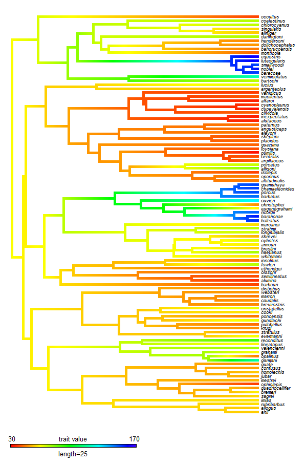
I just posted a new version of the function to plot the posterior density of a binary character mapped on the tree using stochastic character mapping (described
here). The updated code is on the
webpage for phytools, but if you want to use this function version, you are probably better off updating to the most recent, minor release of phytools, v0.2-04,
here. This is because I also had to make some changes to the phytools functions
plotTree,
plotSimmap, and
densityMap, so doing a package update from source is the best way to ensure that you have the correct versions of each function installed.
The biggest difference between this version of
densityMap and the
previous one is that in this version more control of how the plot looks has been migrated to the user. In particular, the user can control the width of plotted edges as well as whether or not to display a fine black outline around the lines of the tree graph. These may seem like minor changes, but to plot the outline I first use
plotTree to plot a tree with
lwd+2 width edges. Then I overlay the
densityMap tree. To do this, I had to modify
plotTree (which is actually just a wrapper for
plotSimmap) so that it could be used to plot multiple trees in the same plotting object. In addition, in previous versions of
plotSimmap, the offset of tip labels is a function of the plotted edge widths. This meant that when I plotted to trees in the same object, but with different width edges, the tip labels did not overlay exactly. The way I fixed this is by migrating control of the label offset to the function arguments - and then I used a label offset based only on the
interior,
densityMap line widths.
Here's an example of the result:
> # install package
> install.packages("phytools_0.2-04.tar.gz",type="source", repos=NULL)
** installing *source* package 'phytools' ...
...
* DONE (phytools)
> library(phytools)
Loading required package: ape
Loading required package: mnormt
...
> # simulate random Yule tree
> tree<-pbtree(n=50,scale=2)
> # simulate data on the tree using sim.history
> Q<-matrix(c(-2,2,2,-2),2,2,dimnames=list(c(0,1),c(0,1)))
> tree<-sim.history(tree,Q)
> # generating stochastic map trees (500, in this case)
> trees<-make.simmap(tree,tree$states,nsim=500)
> # create density map
> densityMap(trees,fsize=c(1,1),outline=TRUE,lwd=6, res=1000)
sorry - this might take a while; please be patient
>
Note that this is pretty slow - to make it quicker, use fewer maps (say 100) or a lower "resolution" (
densityMap argument
res), which is just the number of times the probability/color is sampled along any path from the root to the tips.