extract.clade for tree with a mapped discrete character

A phytools reader recently asked the following via the general comments page:

I have used make.simmap to obtain 1000 stochastic maps for a larger clade. It contains two sister-clades. My main interest is to compare transitions for these two sister-clades. describe.simmap gives average values for the entire clade, while, countSimmap provides number of transitions for 1000 trees. Is there a way to obtain these values individually for sub-clades within phytools, or do I have to run the analyses separately for each sister-clade to obtain these values?

Well, firstly, I would not recommend running stochastic mapping separately for each subtree of interest in your phylogeny - unless you would like to assume that the substitution process for your discrete character is different in different parts of the tree. (Even if it is - unless our subtrees are large then we probably don't have enough information to estimate this difference anyway.) What we'd really like to do is run stochastic mapping on the full tree, and then extract our clades of interest to run describe.simmap on each subtree. Unfortunately - extract.clade from the 'ape' package won't preserve the discrete character mapping on our stochastic mapped tree!

Luckily, there is a solution. phytools does have an analogous function to drop.tip (called drop.tip.simmap), and drop.tip and extract.clade are (in some ways) just the inverse of each other. Let's try to write a mapping compatible version of extract.clade for phylogenies with a mapped discrete character using drop.tip.simmap:

extract.clade.simmap<-function(tree,node){
  x<-getDescendants(tree,node)
  x<-x[x<=length(tree$tip.label)]
  drop.tip.simmap(tree,tree$tip.label[-x])
}

OK, that was easy. Now let's try it:

> Q<-matrix(c(-1,1,1,-1),2,2)
> colnames(Q)<-rownames(Q)<-letters[1:2]
> tree<-sim.history(pbtree(n=100,scale=1),Q)
> cols<-setNames(c("blue","red"),letters[1:2])
> plotSimmap(tree,cols,fsize=0.6,node.numbers=T,lwd=3, pts=F)

Now let's extract the clade descended from node 106 & plot:

> tree106<-extract.clade.simmap(tree,106)
> plotSimmap(tree106,cols,fsize=0.8,lwd=3,pts=F)

Cool.

Note that although the basic functionality is the same, the options and arguments of extract.clade.simmap and extract.clade are not the same.

Version of getCladesofSize that also works for multifurcating trees

As promised earlier, I have figured out how to allow the function getCladesofSize (which gets all the subtrees of a phylogeny that cannot be further subdivided into two subtrees of size greater in size than a specified value) to allow for multifurcating, as well as strictly binary, trees. The updated code is here; and I have also posted a new version of phytools (phytools 0.2-64), which can be downloaded and installed from source.

Here's a quick demo of what the function does:

> require(phytools)
Loading required package: phytools
> packageVersion("phytools")
[1] ‘0.2.64’
> # a tree with lots of polytomies
> plotTree(tree,fsize=0.6)
> is.binary.tree(tree)
[1] FALSE

> trees<-getCladesofSize(tree,5)
> trees
6 phylogenetic trees
> layout(matrix(1:6,3,2))
> plotTree(trees)
Waiting to confirm page change...

Looking at all the trees - we can see that none can be further subdivided into two (or more, for trees polytomous at the root) reciprocally monophyletic groups all containing (in this case) 5 or more tips. Cool.

Extracting all subtrees of a given size & larger

An R-sig-phylo query asked the following:

I'd like to sample independent subclades of greater than N tips from a phylogenetic tree much greater than N, say (number of tips >= 10*N). I can extract all subclades of greater than N taxa, but sampling independent subclades seems to be a harder problem.

Well - I'm not completely sure if this what he's asking for, but here is a function that will get all the subtrees in a binary tree that cannot be further subdivided into two subtrees of size >= clade.size.

getCladesofSize<-function(tree,clade.size=2){
  nn<-1:tree$Nnode+length(tree$tip.label)
  ndesc<-function(tree,node){
    x<-getDescendants(tree,node)
    sum(x<=length(tree$tip.label))
  }
  dd<-setNames(sapply(nn,ndesc,tree=tree),nn)
  aa<-nn[1]
  nodes<-vector()
  while(length(aa)){
    bb<-sapply(aa,function(x,tree)
      tree$edge[which(tree$edge[,1]==x),2],tree=tree)
    cc<-matrix(dd[as.character(bb)],nrow(bb),ncol(bb))
    cc[is.na(cc)]<-1
    gg<-apply(cc,2,function(x,cs)
      any(x < cs),cs=clade.size)
    nodes<-c(nodes,aa[gg])
    aa<-as.vector(bb[,!gg])
  }
  trees<-lapply(nodes,extract.clade,phy=tree)
  class(trees)<-"multiPhylo"
  return(trees)
}

The way this works is as follows. First, we get the number of tips descended from each node in the tree:

nn<-1:tree$Nnode+length(tree$tip.label)
ndesc<-function(tree,node){
  x<-getDescendants(tree,node)
  sum(x<=length(tree$tip.label))
}
dd<-setNames(sapply(nn,ndesc,tree=tree),nn)

Next, we conduct a traversal of the tree from the root. If a node has two daughter clades both of size >= clade.size, then we ascend up the tree to those nodes. If not, then we store the value of the current node. At the end, we extract all subtrees whose node numbers we have stored:

trees<-lapply(nodes,extract.clade,phy=tree)
class(trees)<-"multiPhylo"

That's it.

Right now, the function will only work on binary trees - but there is no check to assure that your tree is binary. I will fix that and add to phytools.

Function to merge mapped states

I just posted a new function (mergeMappedStates) to merge mapped states on a phylogeny with a discrete character map. This is pretty easy. We just do two passes through all the edges of the tree. In the first pass we rename any mapped state in the old states with the new merged state:

rr<-function(map,oo,nn){
  for(i in 1:length(map)) if(names(map)[i]%in%oo)
    names(map)[i]<-nn
  map
}
maps<-lapply(maps,rr,oo=old.states,nn=new.state)

In the second pass, we join any adjacent map elements in the same (new) merged state:

mm<-function(map){
  if(length(map)>1){
    new.map<-vector()
    j<-1
    new.map[j]<-map[1]
    names(new.map)[j]<-names(map)[1]
    for(i in 2:length(map)){
      if(names(map)[i]==names(map)[i-1]){
        new.map[j]<-map[i]+new.map[j]
        names(new.map)[j]<-names(map)[i]
      } else {
        j<-j+1
        new.map[j]<-map[i]
        names(new.map)[j]<-names(map)[i]
      }
    }
    map<-new.map
  }
  map
}
maps<-lapply(maps,mm)

Here's a quick demo of how it works:

> tree<-pbtree(n=100,scale=1)
> Q
   a  b  c
a -2  1  1
b  1 -2  1
c  1  1 -2
> tree<-sim.history(tree,Q)
> plotSimmap(tree,lwd=3,ftype="off",pts=F)
no colors provided. using the following legend:
      a        b        c
 "black"    "red" "green3"

> merged<-mergeMappedStates(tree,c("a","c"),"ac")
> plotSimmap(merged,lwd=3,ftype="off",pts=F)
no colors provided. using the following legend:
    ac      b
"black"  "red"

Cool - seems to work.

New version of rerootingMethod & estimating ancestral states with an ordered model

I just posted a new version of rerootingMethod. This function computes the empirical Bayes posterior probabilities (marginal ancestral state reconstructions) for a discrete character using the re-rooting method of Yang (e.g., Yang 2006). The main functional change in this version is that now the function can take a model index matrix (i.e., a matrix with the same dimensions as Q with integers to specify the different elements to be estimated), instead of just the string "ER" or "SYM". This should allow users to specify any arbitrary symmetric model - not just the full symmetric or equal-rates model.

Our index matrix contains an integer for each rate to be estimated - but values set to zero indicate that the corresponding transition rate should be zero. This caused a little bit of a problem for rerootingMethod because it had the code:

Q<-matrix(YY$rates[YY$index.matrix],ncol(XX),ncol(XX),
 dimnames=list(colnames(XX),colnames(XX)))

This code first creates a vector with the elements of the index matrix; and then coerces that vector into a matrix with dimensions specified by our number of states for the character. The problem is that index matrix elements that are zero will cause the length of the vector to be wrong, so that it cannot be coerced into a matrix with the right dimensions (we're kind of lucky that this is the case - or we might have missed the error). To solve this, I just did:

Q<-matrix(c(0,YY$rates)[YY$index.matrix+1],ncol(XX),
 ncol(XX),dimnames=list(colnames(XX),colnames(XX)))

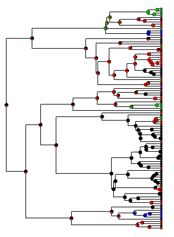
One of the most common symmetric models other than the equal rates model that we might be interested in is probably the ordered model. This is a model in which we, say, allow transition A ⇄ B ⇄ C ⇄ D, but no other types of transitions are allowed. How can we fit this model? Here's a quick demo in which I simulate under the model & then fit it & estimate ancestral states:

> require(phytools)
Loading required package: phytools
> packageVersion("phytools")
[1] ‘0.2.63’
> tree<-pbtree(n=100,scale=2)
> Q<-matrix(c(-1,1,0,0,1,-2,1,0,0,1,-2,1,0,0,1,-1),4,4)
> colnames(Q)<-rownames(Q)<-LETTERS[1:4]
> Q
   A  B  C  D
A -1  1  0  0
B  1 -2  1  0
C  0  1 -2  1
D  0  0  1 -1
> x<-sim.history(tree,Q)$states
> mm<-Q; diag(mm)<-0
> mm
  A B C D
A 0 1 0 0
B 1 0 1 0
C 0 1 0 1
D 0 0 1 0
> aa<-rerootingMethod(tree,x,model=mm)
> plot(tree,no.margin=TRUE,edge.width=2, show.tip.label=FALSE)
> nodelabels(pie=aa$marginal.anc,piecol=palette()[1:4], cex=0.5)
> tiplabels(pie=to.matrix(x,colnames(aa$marginal.anc)), piecol=palette()[1:4],cex=0.3)

Code for the new version of rerootingMethod is here; and the latest phytools build can be downloaded here.

New version of contMap

I just posted a new version of contMap (described here and in my recent MEE article). contMap uses a color scale to map the observed and reconstructed values of a continuous character onto the branches of a phylogeny.

This update just brings contMap into alignment with densityMap in that it (invisibly) returns an object of class "contMap" so that adjusting the plotting parameters can be accomplished without recomputing all the ancestral states.

As I demonstrated on Travis Ingram's recommendation, this - in addition to speeding up re-plotting if we need to change the parameters of our plot - allows us to easily change the palette of colors used to map our trait on the tree. For instance, we can easily change to grayscale. Here I show how we can flip low to high in our color map.

> require(phytools)
Loading required package: phytools
> packageVersion("phytools")
[1] ‘0.2.61’
> tree<-pbtree(n=30)
> x<-fastBM(tree)
> maps<-contMap(tree,x)

Alright, now let's flip the colors:

> maps$cols[]<-maps$cols[length(maps$cols):1]
> plot(maps)

Pretty cool.

Code is here; new phytools build (0.2-61), here.

paintSubTree doesn't actually "paint" the tree (i.e., with colors)

I've been emailing back & forth with a phytools user to try & explain what is done with paintSubTree, plotSimmap, and phylomorphospace with a mapped regime - but I thought some visuals would help & that some other readers (occasional or otherwise) of this blog might find the clarification useful, so I decided to write this quick post.

The first point is that paintSubTree does not paint the tree with colors. The term paint refers to regime painting in Butler & King (2004); i.e., the process of assigning different branches or subtrees to different a priori specified categories or regimes. The states that we choose to assign to these paintings has nothing at all to do with the colors used to visualize the regimes in (for instance) plotSimmap or phylomorphospace, which (if unassigned by the user) are drawn in sequence from palette().

This is what I mean:

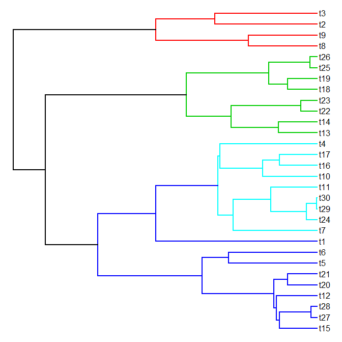
> tree<-pbtree(n=30)
> plotTree(tree,node.numbers=TRUE)

Now let's say we want to paint the subtrees arising from nodes 57, 50, 33, and 42 with different regimes. It doesn't matter why we want to do this - maybe we just want to easily visualize the trees with different subtrees in different colors; nor does it matter that the subtree arising out of node 42 is nested within the subtree arising out of node 33. We can do:

> tree<-paintSubTree(tree,node=57,state="1",anc="0")
> tree<-paintSubTree(tree,node=50,state="2")
> tree<-paintSubTree(tree,node=33,state="3")
> tree<-paintSubTree(tree,node=42,state="4")

Now let's plot the tree with default colors:

> plotSimmap(tree,pts=FALSE)
no colors provided. using the following legend:
      0        1        2        3        4
"black"    "red" "green3"  "blue"  "cyan"

If we want to use different colors, we can just do:

> cols<-c("black","red","blue","green","purple")
> names(cols)<-0:4
> plotSimmap(tree,cols,pts=FALSE)

If our sole purpose in painting on regimes was to visualize the tree in this way, we could have used the desired colors as regimes. I.e.,

> tree<-paintSubTree(tree,node=31,state="black")
> tree<-paintSubTree(tree,node=57,state="red")
> tree<-paintSubTree(tree,node=50,state="blue")
> tree<-paintSubTree(tree,node=33,state="green")
> tree<-paintSubTree(tree,node=42,state="purple")
> cols<-colnames(tree$mapped.edge)
> names(cols)<-cols
> plotSimmap(tree,cols,pts=FALSE)

to exactly the same effect.

Visualizing different regimes in a phylomorphospace works according to the same principle. Here's a quick demo of that using the same tree:

> X<-fastBM(tree,nsim=2)
> phylomorphospace(tree,X,colors=cols,node.by.map=TRUE, xlab="x",ylab="y")

That's really all there is to it.