Monday, December 2, 2013

More on Rphylip: Rdnapars and Rneighbor

I've spent a little more time working on Rphylip. Here are a few updates since my last post: I have now added the functions Rdnapars (for dnapars), Rneighbor (for neighbor). I have also cleaned up the code in various ways by pulling out (for instance) repeated functions like writing a PHYLIP formatted DNA input file, etc.

Perhaps the most interesting addition (in my opinion) - at least for Windows users who work in R - is the addition of an internal function findPath. (See code here.) This function means that users of Rphylip may no longer be required to specify the path to the directory containing the PHYLIP executable files. Instead, if no path is supplied, R will check various places on the computer where it is likely to be found (for instance the current working directory, C:\Program Files\", etc.). To my surprise, this option works surprisingly well - and also does not bomb R if the directory containing PHYLIP cannot be found (instead returning a sensible error message).

For instance, witness the following example in which PHYLIP is hidden:

> require(Rphylip)
Loading required package: Rphylip
Loading required package: ape
> data(primates)
> tree<-Rdnapars(primates)
Error in Rdnapars(primates) :
No path provided and was not able to find path to dnapars

OK, now let's put the PHYLIP folder back someplace sensible, in this case in C:/Program Files:

> tree<-Rdnapars(primates)
...

DNA parsimony algorithm, version 3.695


One most parsimonious tree found:


                                     +----12   
                                 +--10 
                            +----9   +------11
                            |    | 
                       +----8    +-----10
                       |    | 
                  +----7    +--------9
                  |    | 
            +-----6    +----------8    
            |     | 
            |     |       +------7    
            |     +-------5 
            |             |    +-----6    
  +---------2             +----4 
  |         |                  |  +---5  
  |         |                  +--3 
  |         |                     +-4   
  |         | 
  |         +------------3        
  | 
  1---------------2        
  | 
  +-------------1        


requires a total of    593.000

...

Translation table
-----------------
        1       Lemur
        2       Tarsier
        3       Sq.Monkey
        4       J.Macaque
        5       R.Macaque
        6       E.Macaque
        7       B.Macaque
        8       Gibbon
        9       Orangutan
        10      Gorilla
        11      Chimp
        12      Human

> plot(tree,edge.width=2,no.margin=TRUE)

That worked.

Rphylip is also now on GitHub - so you can follow updates & changes to the code there.

Saturday, November 30, 2013

New project - Rphylip: an R interface for PHYLIP

Just towards the end of this week I started working on a new project, Rphylip, which is designed to provide an R interface for the longstanding, popular phylogenetics package PHYLIP. PHYLIP does a really remarkable number of different analysis - from a wide range of phylogeny inference methods, to a variety of comparative methods (including several important new approaches that are implemented nowhere else), to tree drawing and other things. A complete list of the programs in the PHYLIP package is here.

My goal is to create functions that interface with the programs of PHYLIP, but allow the user to operate completely within R. That is, all inputs for the PHYLIP programs are created by R; and all outputs are parsed back into R or printed to the R console. Finally, Rphylip will even clean up the input & output files it has created for the PHYLIP programs.

So far, I have created test functions to interface with only a few of the programs of PHYLIP: Rdnaml (for dnaml); Rcontml (for contml; and Rcontrast (for contrast).

To use Rphylip one has to, of course, first install PHYLIP on your computer. Having done this, it is straightforward to run any of the programs of PHYLIP through R. Below is a simple demo using Rdnaml under the default conditions (which are slightly different then the defaults for dnaml). Some output excluded:

> require(Rphylip)
Loading required package: Rphylip
Loading required package: ape
> X<-read.dna("primates.dna")
> X
12 DNA sequences in binary format stored in a matrix.

All sequences of same length: 232
Labels: Lemur Tarsier Sq.Monkey J.Macaque R.Macaque E.Macaque ...

Base composition:
    a     c     g     t
0.364 0.414 0.041 0.181

> tree<-Rdnaml(X,path="C:/Users/Liam/phylip/exe")
Warning:
  One or more of "infile", "outfile", "outtree"
  was found in your current working directory and may be overwritten

Press ENTER to continue or q to quit:

...

Nucleic acid sequence Maximum Likelihood method, version 3.695

...

               +--------------3
               | 
               |          +--------8
               |          | 
               |          |          +-----11
  +------------8    +-----2       +--1 
  |            |    |     |    +--3  +--12
  |            |    |     |    |  | 
  |            |    |     +----5  +----10 
  |            |    |          | 
  |            +----4          +--------9 
  |                 | 
  |                 |              +4    
  |                 |           +-10 
  |                 |        +--6  +--5  
  |                 |        |  | 
  |                 +--------7  +--6 
  |                          | 
  |                          +------7 
  | 
  9-------------------2        
  | 
  +------------------1

remember: this is an unrooted tree!
...

Translation table
-----------------
        1       Lemur
        2       Tarsier
        3       Sq.Monkey
        4       J.Macaque
        5       R.Macaque
        6       E.Macaque
        7       B.Macaque
        8       Gibbon
        9       Orangutan
        10      Gorilla
        11      Chimp
        12      Human

> tree$logLik
[1] -2200.766
> require(phangorn)
Loading required package: phangorn
Loading required package: rgl
> plot(midpoint(tree),edge.width=2,no.margin=TRUE)

The source code for the functions I've written so far in Rphylip are here and I posted a little package build with some minimal documentation for the three interface functions here: http://www.phytools.org/Rphylip/. Feedback welcome!

Difference between gammaStat & ltt when the tree is slightly non-ultrametric

A phytools user reported a small, but measurable, difference in Pybus & Harvey's γ computed by gammaStat in ape and ltt in the phytools package. Since I know that ltt and gammaStat return the same value of γ for trees that are genuinely ultrametric, my guess was that the tree might not be precisely ultrametric. In fact, this turns out to be the case. Even though the tree passed the check is.ultrametric, trees can only be ultrametric to the degree of numerical precision that can be represented in the computer, and trees that are read in from file will generally be still considerably more non-ultrametric than that (due to rounding in the input file).

The user was kind enough to send me her tree so I was able to verify that this was indeed the case. The tree passes the check of is.ultrametric, but as we decrease tol, it eventually fails. Furthermore, it turns out to be the case that γ reported by gammaStat for a slightly non-ultrametric tree is exactly the same as a precisely ultrametric tree where all the tips have the same height as the highest tip; and γ reported by ltt for a slightly non-ultrametric tree is (nearly) exactly the same as for a precisely ultrametric tree where all the tips have the same height as the lowest tip. Here's how I found out (using the problematic tree):

> tree<-read.nexus("Trees.nex")
> gammaStat(tree)
[1] 2.320419
> ltt(tree,plot=FALSE)$gamma
[1] 2.321524
>
> ## compute the heights of all tips
> H<-nodeHeights(tree)
> h<-sapply(1:length(tree$tip.label),function(ii,h,e) h[which(e==ii)],h=H[,2],e=tree$edge[,2])
>
> ## the difference from the max height
> d<-max(h)-h
> ## add each difference to the tip
> for(i in 1:length(d))
+ tree$edge.length[which(tree$edge[,2]==i)] <- tree$edge.length[which(tree$edge[,2]==i)]+d[i]
>
> ## now they're the same & equal to gammaStat
> gammaStat(tree)
[1] 2.320419
> ltt(tree,plot=FALSE)$gamma
[1] 2.320419
>
> ## start again
> tree<-read.nexus("Trees.nex")
> gammaStat(tree)
[1] 2.320419
> ltt(tree,plot=FALSE)$gamma
[1] 2.321524
>
> ## the difference from the min
> d<-min(h)-h
> ## add each difference to the tip
> for(i in 1:length(d))
+ tree$edge.length[which(tree$edge[,2]==i)] <- tree$edge.length[which(tree$edge[,2]==i)]+d[i]
>
> ## now they're the same & equal to ltt
> gammaStat(tree)
[1] 2.321529
> ltt(tree,plot=FALSE)$gamma
[1] 2.321529

I just posted a new version of ltt that first checks that the tree is ultrametric & then if it passes is.ultrametric then it corrects the tree to be precisely ultrametric so that the computed γ lines up with gammaStat.

Wednesday, November 27, 2013

Plotting the number of steps under parsimony to attach a new tip to all possible places in a tree

A few days ago, I received an email with the following text:

"What I have been trying to do is to color the branches of a tree according to the number of steps under parsimony that are required if certain species is attached to the corresponding branch of a backbone tree. As I am paleontologist, I usually need to place certain morphological-defined species onto a backbone constraint tree. But I could not find yet the function to do that. Any help is appreciated!"

Like many such emails (unfortunately) I flagged it to (hopefully) return to later, and then I rediscovered it today. Upon closer look, my first reaction was "why do people think I know how to do these things?" As I started to respond as such, it struck me that in fact this shouldn't be that hard (thanks, in large part, to Klaus Schliep's great package phangorn).

First, let's simulate the empirical case in which the 'backbone' tree for our N taxa is 'known', but we have data for N+1 taxa and we want to know where that extra tip belongs:

## load libraries
require(phytools)
require(phangorn)

## simulate tree
tt<-pbtree(n=26,tip.label=LETTERS[26:1])
## this is our true, full, unrooted phylogeny
plot(unroot(tt),use.edge.length=FALSE,type="unrooted", edge.width=2)
## simulate data on the true tree
X<-genSeq(tt,l=2000,format="phyDat",rate=0.01)
## now let's drop one of our tips, tip "Z" in this case
tree<-drop.tip(tt,LETTERS[26])
tree<-unroot(tree) # unroot

OK, now we have a data set (X) containing 26 taxa; but an unrooted tree (tree) containing only 25 tips, and we want to know (& plot) the change in parsimony score that results from attaching the one remaining tip to all of the 48 places in the tree to which it could be attached!

## first set all branch lengths to 1.0
## this is just for bind.tip
tree$edge.length<-rep(1,nrow(tree$edge))
## vector for parsimony scores
ps<-vector(length=nrow(tree$edge))
names(ps)<-apply(tree$edge,1,paste,collapse=",")
## tip to attach
tip.label<-LETTERS[26]
## loop over all edges in the tree
for(i in 1:nrow(tree$edge)){
  ## attach tip
  x<-bind.tip(tree,tip.label,1,where=tree$edge[i,2],
    position=0.5)
  x$edge.length<-NULL
  ## compute parsimony score
  ps[i]<-parsimony(x,X)
}
## subtract parsimony score on 25-taxon tree
ps<-ps-parsimony(tree,X)

Let's see what ps (the parsimony cost of attaching the tip to all edges of the tree) looks like in this one case:

> ps
 26,1 26,27  27,2  27,3 26,28  28,4 28,29 29,30  30,5
  121   122   172   172    97   124   121   146   178
30,31 31,32  32,6  32,7  31,8 29,33 33,34 34,35 35,36
  178   211   211   212   211   147   149   155   168
 36,9 36,10 35,37 37,38 38,11 38,12 37,13 34,39 39,40
  216   216   169   212   224   222   210   153   183
40,41 41,14 41,15 40,16 39,42 42,43 43,44 44,17 44,18
  202   216   216   203   183   210   210   217   217
43,19 42,20 33,45 45,46 46,47 47,21 47,22 46,23 45,48
  209   209   148   200   219   235   235   219   200
48,24 48,25
  216   218

names(ps) here gives the starting & ending node numbers for each edge in the tree & ps its corresponding parsimony cost.

The neatest thing is that we can easily plot these on the tree using the phytools function plotBranchbyTrait (which, unlike other plotting functions in phytools, calls the ape function plot.phylo internally):

plotBranchbyTrait(tree,ps,type="unrooted",prompt=TRUE, title="parsimony cost")

It's pretty clear that the cost of attaching tip "Z" is indeed lowest along the edge (the internode connecting the terminal edges leading to tips "V" and "Y") where tip "Z" actually belongs. Cool.

Note that if we had a model for the evolution of our characters (in this case, our data are DNA sequences - but the query pertained to morphological data from fossils so this is not guaranteed) we could easily construct a similar plot showing differences in the likelihood across the tree.

That's it.

Tuesday, November 26, 2013

Bug fix for phenogram(...,spread.labels=TRUE) for when labels don't actually overlap

I just discovered a small bug in phenogram (the phytools function for plotting traitgrams in various ways) which causes phenogram(...,spread.labels=TRUE) to fail when labels actually don't overlap. So, for instance:

> library(phytools)
> tree<-pbtree(n=10,tip.label=LETTERS[10:1])
> ## no problem
> phenogram(tree,setNames(1:10,tree$tip.label))
> ## problem
> phenogram(tree,setNames(1:10,tree$tip.label), spread.labels=TRUE)
Error in optim(zz, ff, yy = yy, mo = mo, ms = ms, cost = cost, method = "L-BFGS-B", :
L-BFGS-B needs finite values of 'fn'

The bug is because if the labels do not overlap at all when we start our optimization to minimize overlap, the objective function becomes undefined. The fix just checks to ensure that there is some overlap, and if not spits back the original vertical positions of the tip labels.

> source("http://www.phytools.org/phenogram/v1.1/phenogram.R")
> ## fixed
> phenogram(tree,setNames(1:10,tree$tip.label), spread.labels=TRUE)

I also changed the default spread.cost, which controls how much to penalize overlap & deviation from the vertical position, x, respectively; although this is still totally under user control.

Bug fix for anc.Bayes

phytools has a function, anc.Bayes, for ancestral state estimation of continuous traits using Bayesian MCMC. In preparing a tutorial on ancestral character estimation for my phylogeny methods graduate class, I uncovered a serious error in how the prior probability was calculated. I have now fixed it and posted the code, along with a new phytools build (phytools 0.3-79) that contains this fix.

If you used anc.Bayes with an uninformative prior, this bug probably did not affect you. However, if you tried a strong informative prior in your analysis, then prior versions of this function will not have worked properly.

I also (re-) discovered that the way this function handles specification of the prior and other control parameters of the MCMC is pretty annoying. The function is probably due an overhaul! Hopefully, I can get to that at some point.

Saturday, November 23, 2013

Cool use of densityMap and contMap (& in the same figure!)

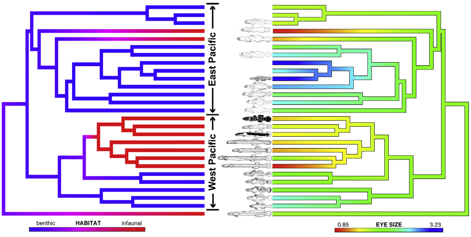
I just learned of this recent article by Ryan Ellingson et al. which makes very neat use of the phytools functions densityMap and contMap for plotting a posterior density from stochastic mapping on a tree, and for mapping a continuous character on the tree (respectively). See Revell (2013) for more details. Below is a reproduction of their figure. On the left is a posterior density from stochastic mapping of 'benthic' vs. 'infaunal' habit; whereas on the right is a projection of the observed or reconstructed values of a continuous character, relative eye size. For more details see the original article, Ellingson et al. (2013).

Click here for larger version.

**Disclaimer: neither densityMap nor contMap can be used (directly) to add tiny line images of fishes to your tree!