I just posted code for a new function that conducts the phylogenetic paired t-test of Lindenfors et al. (2010; of which I am also a co-author). Since I am out in the field here on Staniel Cay Exuma, in the Bahamas, it is somewhat difficult for me to error check, etc., so I leave that to my readers. . . . Just kidding, I'm pretty sure there is no major problems with this function, but I am (as always) happy to hear any feedback.
The phylogenetic paired t-test we used in our study was really pretty simple. Basically, we just computed the so-called "phylogenetic mean" for the difference between two values in each species (in our study, these were physiological measures collected from males and females of primates), and we asked if the mean difference was significantly different from zero. In addition, we also incorporated uncertainty about the species means for each trait (essentially following Ives et al. 2007); and we optimized Pagel's λ for the difference.
To use the function, first download it (my R-phylogenetics page; direct link to code here) and load from source; then type:
> result<-phyl.pairedttest(tree,x1,x2)
The result is a list which contains the mean difference, the optimized value of lambda, and some other things.
With a little creativity, this function can also be used to test the hypothesis that the phylogenetic mean for a single trait or a difference between traits is significantly different from an arbitrary value; or to evaluate the phylogenetic signal for a single trait or the difference between two traits.
More soon. . . .
Thursday, May 26, 2011

Sunday, May 22, 2011
Fitting two or more evolutionary correlations to the tree and data
As of late, I am in the field and haven't had time to do much coding (although I am slowly working on implemented the phylogenetic paired t-test of my article with Patrik Lindenfors and Charlie Nunn); however, I thought I would create a quick note about a function that I have available on my R-phylogenetics page, but that I have not described in any earlier blog posts.
The function evol.vcv() fits the model of Revell & Collar (2009). In this article we fit two different BM variance-covariance matrices (we call these "evolutionary rate matrices" - because the diagonal elements are the evolutionary rates, by some account), to different parts of the tree that have been specified a priori by the user. In my implementation (direct link to code here), the user can fit an arbitrary number of traits as well as an arbitrary number of rate matrix categories. These are "painted" on the tree using SIMMAP v1.0 format Newick trees that are read into memory using the function read.simmap() (code here; prior descriptions of the development of this function in several posts).
One of the neat things about this model is that it allows the user to fit different evolutionary correlations between characters to different branches and parts of branches in the tree. For instance, in our study we fit this model for piscivorous and non-piscivorous fish species and found that the evolutionary correlation between two different aspects of buccal morphology was much higher in piscivorous fish species.
To try the function, first load the source:
> source("http://faculty.umb.edu/liam.revell/phytools/evol.vcv/v0.1/evol.vcv.R") # or download
Then, simply read in a data matrix, X, which can contain an arbitrary number of columns, e.g.:
> X<-read.csv(file="data.csv",row.names=1)
Then read the tree in simmap v1.0 format:
> tree<-read.simmap(file="treefile.tre",format="nexus") # for instance
Finally, execute the analysis:
> result<-evol.vcv(tree,X,maxit=5000)
The output is the fit and fitted parameters of both a one matrix and two evolutionary rate matrix model, as well as a comparison of the models.
The function evol.vcv() fits the model of Revell & Collar (2009). In this article we fit two different BM variance-covariance matrices (we call these "evolutionary rate matrices" - because the diagonal elements are the evolutionary rates, by some account), to different parts of the tree that have been specified a priori by the user. In my implementation (direct link to code here), the user can fit an arbitrary number of traits as well as an arbitrary number of rate matrix categories. These are "painted" on the tree using SIMMAP v1.0 format Newick trees that are read into memory using the function read.simmap() (code here; prior descriptions of the development of this function in several posts).
One of the neat things about this model is that it allows the user to fit different evolutionary correlations between characters to different branches and parts of branches in the tree. For instance, in our study we fit this model for piscivorous and non-piscivorous fish species and found that the evolutionary correlation between two different aspects of buccal morphology was much higher in piscivorous fish species.
To try the function, first load the source:
> source("http://faculty.umb.edu/liam.revell/phytools/evol.vcv/v0.1/evol.vcv.R") # or download
Then, simply read in a data matrix, X, which can contain an arbitrary number of columns, e.g.:
> X<-read.csv(file="data.csv",row.names=1)
Then read the tree in simmap v1.0 format:
> tree<-read.simmap(file="treefile.tre",format="nexus") # for instance
Finally, execute the analysis:
> result<-evol.vcv(tree,X,maxit=5000)
The output is the fit and fitted parameters of both a one matrix and two evolutionary rate matrix model, as well as a comparison of the models.
Sunday, May 15, 2011
Field work in the Bahamas
Research in my lab (of one at the moment - but we soon shall be more) takes place in two main areas: computational method development for evolutionary biology; and evolutionary ecology of lizards. The latter calling has me blogging in absentia tonight as I have joined my former Ph.D advisor, Jonathan Losos, and several other colleagues on a 2.5 week field trip to Staniel Cay in the Bahamas. To read more about Jonathan's twenty years (and counting) of field work in the Bahamas, see his blog post here.
Friday, May 13, 2011
New version of optim.phylo.ls()
I just posted a new version of optim.phylo.ls(). This function is for phylogeny inference using the least-squares method. According to this method, we find the tree and branch lengths for which the sum of squared differences between the observed (e.g., measured from DNA sequences) and implied (i.e., the patristic distances on the tree) is minimized. Direct link to code for the new version (v0.4) is here.
My updates arose out of a R-sig-phylo thread on recovering lost branch lengths from a tree when all one has is the topology and a patristic distance matrix. This can be done using the least-squares method (and, in fact, here we are guaranteed to recover the true branch lengths, as noted in Felsenstein 2004). I now make it easy to do so by introducing the option fixed=TRUE which just uses the input tree and stops the inference machinery (which relies on nni() from the {phangorn} package) from running. More on all of this later if I have time.
As an aside - widespread problems with blogger.com means that a post I created yesterday has disappeared! Luckily, I saved a copy (actually, I did this by tracking it down in Google's cache when I first noticed it vanish). I will repost this later if it doesn't reappear on its own.
My updates arose out of a R-sig-phylo thread on recovering lost branch lengths from a tree when all one has is the topology and a patristic distance matrix. This can be done using the least-squares method (and, in fact, here we are guaranteed to recover the true branch lengths, as noted in Felsenstein 2004). I now make it easy to do so by introducing the option fixed=TRUE which just uses the input tree and stops the inference machinery (which relies on nni() from the {phangorn} package) from running. More on all of this later if I have time.
As an aside - widespread problems with blogger.com means that a post I created yesterday has disappeared! Luckily, I saved a copy (actually, I did this by tracking it down in Google's cache when I first noticed it vanish). I will repost this later if it doesn't reappear on its own.
Thursday, May 12, 2011
Issue with extract.clade() relevant to evol.rate.mcmc()
Paolo Piras just clued me into an issue with the {ape} function extract.clade() that affects the pre-processing of the posterior sample from our two-rate Bayesian MCMC analysis performed using evol.rate.mcmc(). Basically, for some orderings of the $edge matrix (in particular, the "cladewise" order given by {phangorn} functions), extract.clade() appears to scramble the tip labels under certain conditions.
For instance, from Paolo's example (but with tip labels altered) if we take the following tree (with nodes labeled according to their indexes in phy$edge):

then extract the clade descended from node "35" and plot it:
> tr<-extract.clade(phy,node=35)
> plot(tr)
we get the following:

Uh-oh - for some reason the tip species "R" & "V" and "T" & "X" have been swapped in the extracted clade!!
It turns out that the easiest way to resolve this is by first computing:
> phy<-read.tree(text=write.tree(phy))
which will guarantee that extract.clade() works properly for this problem. One thing to note, though, is that doing so will change the indexes for the nodes in $edge. Thus, it is essential that this be done before running evol.rate.mcmc() and not after evol.rate.mcmc() but before posterior.evolrate(). I am presently trying to figure out what the smartest way to build this into evol.rate.mcmc() would be.
As an aside, though, this bug is not lethal to evol.rate.mcmc() as the specific ordering of the tip labels in the extracted subtree is not used by posterior.evolrate() (although creating the plotting given here will be affected).
For instance, from Paolo's example (but with tip labels altered) if we take the following tree (with nodes labeled according to their indexes in phy$edge):

then extract the clade descended from node "35" and plot it:
> tr<-extract.clade(phy,node=35)
> plot(tr)
we get the following:

Uh-oh - for some reason the tip species "R" & "V" and "T" & "X" have been swapped in the extracted clade!!
It turns out that the easiest way to resolve this is by first computing:
> phy<-read.tree(text=write.tree(phy))
which will guarantee that extract.clade() works properly for this problem. One thing to note, though, is that doing so will change the indexes for the nodes in $edge. Thus, it is essential that this be done before running evol.rate.mcmc() and not after evol.rate.mcmc() but before posterior.evolrate(). I am presently trying to figure out what the smartest way to build this into evol.rate.mcmc() would be.
As an aside, though, this bug is not lethal to evol.rate.mcmc() as the specific ordering of the tip labels in the extracted subtree is not used by posterior.evolrate() (although creating the plotting given here will be affected).
Tuesday, May 10, 2011
Bug fix in ltt()
One of my Phylogenetics students, Craig Sadowski, just found a bug in the latest version of my function ltt() which computes and creates a lineage-through-time plot; as well as calculating and hypothesis testing the γ statistic of Pybus & Harvey (2000). Basically, when I moved tol (a tolerance value for rounding) out of the function call, I neglected to assign it a value. Oops. Fixed in v0.5 (code here).
Parameter estimates from evol.rate.mcmc()
My coauthors (1,2,3) and I are nearing completion of the revisions for the manuscript describing our MCMC method for identifying the location of a shift in the evolutionary rate through time. I have described the approach and our methods for collapsing the posterior sample in several prior posts (e.g., 1,2,3,4,5,6,7).
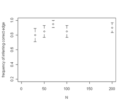
Among the interesting results that have been revealed so far - for a given rate shift our capacity to identify the correct edge on the tree where the rate shift occurred seems to be fairly insensitive to the total size of the tree. For instance, the plot below is for trees of size ranging from N=30 through N=200:
However, we have also found that the ratio of estimated rates (i.e., σ22/σ12) is downwardly biased for small trees, e.g., from an example in which the generating rate ratio σ22/σ12=10:
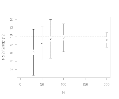
In other words, for small trees the estimated evolutionary rates are too similar relative to the generating rates. We believe, and explain in our manuscript, that this is a direct consequence of integrating across uncertainty in the location of the rate shift (thanks to BR for this insight). For a given rate shift, the posterior density for the location of the shift tends to be much more diffuse on a smaller tree. It makes sense therefore that the estimated difference in evolutionary rates (here, the ratio) will be downwardly biased because we have many posterior samples on incorrect branches where (at least on one side of this split) low and high rates are averaged.
By the way, the plots above were created using plotCI() from the {gplots} package.
More on this and more minor updates to evol.rate.mcmc() (latest version here) coming soon.
Among the interesting results that have been revealed so far - for a given rate shift our capacity to identify the correct edge on the tree where the rate shift occurred seems to be fairly insensitive to the total size of the tree. For instance, the plot below is for trees of size ranging from N=30 through N=200:

However, we have also found that the ratio of estimated rates (i.e., σ22/σ12) is downwardly biased for small trees, e.g., from an example in which the generating rate ratio σ22/σ12=10:

In other words, for small trees the estimated evolutionary rates are too similar relative to the generating rates. We believe, and explain in our manuscript, that this is a direct consequence of integrating across uncertainty in the location of the rate shift (thanks to BR for this insight). For a given rate shift, the posterior density for the location of the shift tends to be much more diffuse on a smaller tree. It makes sense therefore that the estimated difference in evolutionary rates (here, the ratio) will be downwardly biased because we have many posterior samples on incorrect branches where (at least on one side of this split) low and high rates are averaged.
By the way, the plots above were created using plotCI() from the {gplots} package.
More on this and more minor updates to evol.rate.mcmc() (latest version here) coming soon.
Subscribe to:
Posts (Atom)