Just a quick tidbit about unloading a library from the current R session using detach().
Say we have a current session of R open, and, lo and behold, there is a new version of "phytools" available. If we download the binaries and try to install, e.g.:
> install.packages("phytools_0.0-3.zip",repos=NULL)
we get the following error:
Warning: package 'phytools' is in use and will not be installed
This can be avoided simply by unloading the library before installing, and the reloading the new version afterwards. This is accomplished as follows:
> detach(package:phytools)
> install.packages("phytools_0.0-3.zip",repos=NULL)
package 'phytools' successfully unpacked and MD5 sums checked
> require(phytools)
Loading required package: phytools
Of course, this also applies to packages installed from a CRAN mirror.
Wednesday, June 29, 2011

Tuesday, June 28, 2011
Slicing a tree to create all subtrees
Someone recently emailed me about slicing a tree at a particular height from the root and then keeping all the subtrees. This seemed pretty easy, so I thought I would implement it using the {ape} function extract.clade(). This is how I did it. First, I reordered the tree "cladewise", using reorder.phylo(); next, I computed the heights of all the internal and terminal nodes in the tree and put these values into a matrix to match the $edge matrix from my "phylo". Then, I found all the edges intersected by my slice and identified the tipward nodes on those edges, excluding all the nodes that were also tips. Finally, I extracted each subtree descended from the nodes using extract.clade() and added a $root.edge to each tree depending on where its root branch was sliced. I then returned all of these trees as a "multiPhylo" object.
The function is posted to my website, here. Please be warned that I'm not sure what will happen if the slice point is greater than the tree length or if it only intersects terminal edges.
First, let's create a random tree:
> require(geiger)
> tree<-birthdeath.tree(b=1,d=0,taxa.stop=20)

Now, let's slice it at slice=0.6, shown as the dotted line above (having verified, of course, that this will indeed produce some non-trivial subtrees):
> source("treeSlice.R")
> trees<-treeSlice(tree,0.6)
> plot(trees,root.edge=T)
which, in this case, produces the following set of three trees:

We're done!
The function is posted to my website, here. Please be warned that I'm not sure what will happen if the slice point is greater than the tree length or if it only intersects terminal edges.
First, let's create a random tree:
> require(geiger)
> tree<-birthdeath.tree(b=1,d=0,taxa.stop=20)

Now, let's slice it at slice=0.6, shown as the dotted line above (having verified, of course, that this will indeed produce some non-trivial subtrees):
> source("treeSlice.R")
> trees<-treeSlice(tree,0.6)
> plot(trees,root.edge=T)
which, in this case, produces the following set of three trees:

We're done!
plotSimmap() & make.simmap() added to new version of "phytools"
I just posted a new version (0.0-3) of the "phytools" package (still in "alpha" release from my website only). This version contains a couple of minor updates as well as the addition of make.simmap() (to generate stochastic character mapped trees) and plotSimmap() (to plot them), both of which I hope prove to be handy functions.
Anolis biogeography stochastically mapped on the Caribbean phylogeny
I thought I would give both make.simmap() and plotSimmap() a practical go, so I decided to map & plot a plausible scenario for island colonization in the Caribbean - shown below:
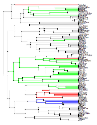
[Click here for higher resolution version.]
I made a couple of updates to both make.simmap() and plotSimmap() to make this possible.
First, in the ML transition matrix, estimated inside make.simmap() using ace(), some of the transition rates were 0.0 in the full, symmetric model for these data. This makes sense, given the large number of states (four - for the four main islands in the Greater Antilles) and small number of transitions between states. I decided to allow additional models - in this case, using the equal-rates model:
> mtree<-make.simmap(tree,x,model="ER")
Next, plotting a relatively large tree created some graphical problems. First, I eliminated all the whitespace around the plot by setting the graphical parameter, par()$mar within the function:
par(mar=c(0.1,0.1,0.1,0.1))
Finally, I added the option to manipulate the font size for the tip labels. This just changes the graphical parameter cex.
> plotSimmap(mtree,fsize=0.7)
for instance.
I will shortly post these updated versions of make.simmap() and plotSimmap() to my R phylogenetics page and I will add them to the next version of "phytools."

[Click here for higher resolution version.]
I made a couple of updates to both make.simmap() and plotSimmap() to make this possible.
First, in the ML transition matrix, estimated inside make.simmap() using ace(), some of the transition rates were 0.0 in the full, symmetric model for these data. This makes sense, given the large number of states (four - for the four main islands in the Greater Antilles) and small number of transitions between states. I decided to allow additional models - in this case, using the equal-rates model:
> mtree<-make.simmap(tree,x,model="ER")
Next, plotting a relatively large tree created some graphical problems. First, I eliminated all the whitespace around the plot by setting the graphical parameter, par()$mar within the function:
par(mar=c(0.1,0.1,0.1,0.1))
Finally, I added the option to manipulate the font size for the tip labels. This just changes the graphical parameter cex.
> plotSimmap(mtree,fsize=0.7)
for instance.
I will shortly post these updated versions of make.simmap() and plotSimmap() to my R phylogenetics page and I will add them to the next version of "phytools."
Plot stochastic character mapped tree
I just completed a beta version of my plotSimmap() function. I'll post a little more about how this was accomplished tomorrow, but it was fairly straightforward after figuring out how to plot rooted phylograms generally (see previous post here). To check it out, download it (source here), load the source into R, and then run the following code (for example):
> require(geiger)
> require(phytools)
> tree<-drop.tip(birthdeath.tree(b=1,d=0,taxa.stop=21),"21")
> x<-sim.char(tree,model.matrix=list(matrix(c(-1,1,1,-1),2,2)),
model="discrete")[,,1]
> mtree<-make.simmap(tree,x)
> legend<-c("red","yellow"); names(legend)<-c(1,2)
> source("plotSimmap.R")
> plotSimmap(mtree,legend)
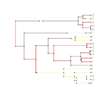
It might also be a good to download the latest version of make.simmap() because there may be a bug in the previous version. I'll add these updates to the next version of {phytools}.
> require(geiger)
> require(phytools)
> tree<-drop.tip(birthdeath.tree(b=1,d=0,taxa.stop=21),"21")
> x<-sim.char(tree,model.matrix=list(matrix(c(-1,1,1,-1),2,2)),
model="discrete")[,,1]
> mtree<-make.simmap(tree,x)
> legend<-c("red","yellow"); names(legend)<-c(1,2)
> source("plotSimmap.R")
> plotSimmap(mtree,legend)

It might also be a good to download the latest version of make.simmap() because there may be a bug in the previous version. I'll add these updates to the next version of {phytools}.
Monday, June 27, 2011
Plotting rooted trees
Now that I have a function to generate stochastic character mapped trees, I thought I would try and see if there would be an easy way to plot them - that is without having to first transform the tree object into another format. [For instance, if I printed the tree to file, I could then read it into FigTree, which I believe can plot mutationally mapped trees; similarly, Rich Fitzjohn tells me that {diversitree} has SIMMAP plotting capabilities.]
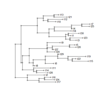
To venture down this road, I first had to try to figure out how trees are plotted. I'll be the first to admit that this is largely untrodden territory for me (with the possible exception of my phylomorphospace plotting function). This was this morning's adventure, and I have just posted a function, plotTree(), which (if not pretty) seems to do the trick.
A few comments on the process. First, getting the lengths of edges, as well as their horizontal positions, is easy. In fact, I had already solved this in an earlier function. Second, the tricky part was figuring out vertical spacing and ordering. Some clues about how to do this are helpfully provided in Felsenstein's (2004) book chapter on plotting trees. This proved to be invaluable in the end.
The way we do this is first by reordering the tree "cladewise" (using reorder.phylo() from the {ape} package) and then spacing the tips of the tree out evenly. The height of all the terminal edges is now assigned. Next, we reorder the tree "pruningwise" - this allows us to now go from the tips of the tree to the root, encountering each internal node before its predecessor. Each time, we assign a vertical position for that node (and the corresponding preceding edge) as the average position of the two descendants, in a binary tree (or the average of the first and the last in a tree with multifurcations). This is the "intermediate" algorithm given by Felsenstein (2004; p. 574) Finally, we connect all the horizontal edges with vertical lines, and add tip labels if inclined.
Even though this plotting function just does more or less the same thing (but slower) as {ape}'s plot.phylo(), I have posted the code here for interested readers. Example execution code and plot are given below:
> require(ape)
> source("plotTree.R")
> tree<-rtree(25)
> plotTree(tree)
To venture down this road, I first had to try to figure out how trees are plotted. I'll be the first to admit that this is largely untrodden territory for me (with the possible exception of my phylomorphospace plotting function). This was this morning's adventure, and I have just posted a function, plotTree(), which (if not pretty) seems to do the trick.
A few comments on the process. First, getting the lengths of edges, as well as their horizontal positions, is easy. In fact, I had already solved this in an earlier function. Second, the tricky part was figuring out vertical spacing and ordering. Some clues about how to do this are helpfully provided in Felsenstein's (2004) book chapter on plotting trees. This proved to be invaluable in the end.
The way we do this is first by reordering the tree "cladewise" (using reorder.phylo() from the {ape} package) and then spacing the tips of the tree out evenly. The height of all the terminal edges is now assigned. Next, we reorder the tree "pruningwise" - this allows us to now go from the tips of the tree to the root, encountering each internal node before its predecessor. Each time, we assign a vertical position for that node (and the corresponding preceding edge) as the average position of the two descendants, in a binary tree (or the average of the first and the last in a tree with multifurcations). This is the "intermediate" algorithm given by Felsenstein (2004; p. 574) Finally, we connect all the horizontal edges with vertical lines, and add tip labels if inclined.
Even though this plotting function just does more or less the same thing (but slower) as {ape}'s plot.phylo(), I have posted the code here for interested readers. Example execution code and plot are given below:
> require(ape)
> source("plotTree.R")
> tree<-rtree(25)
> plotTree(tree)

Friday, June 24, 2011
New version of phytools; PDF manual
I just added the function make.simmap() and the latest version of brownie.lite() to {phytools} and posted the updated version online here. I also fixed a bunch of errors in the help files. In addition, I have posted the phytools PDF manual (which basically just compiles the DESCRIPTION file and all the help pages) here. Please feel free to post feedback or comments.
Subscribe to:
Posts (Atom)