REML version of brownie.lite

I just posted a new, simplified REML version of brownie.lite(). brownie.lite() is based on the method of O'Meara et al. (2006) in which we fit different evolutionary rates to different, pre-defined parts of a phylogenetic tree with branch lengths.

The REML version works by using a likelihood function for the phylogenetically independent contrasts rather than for the original data. We optimize the multi-rate model, in this case, by optimization the (restricted) likelihood of different rescaling of the different branch lengths of the tree. The problem with maximizing the likelihood for the original data is that it involves constructing and inverting matrices of dimension n×n for n species. By maximizing a likelihood function for the contrasts, we can avoid this very computationally intensive operation. In addition, REML (unlike ML) produces unbiased parameter estimates. ML estimates are biased downward by a factor of n/(n-1).

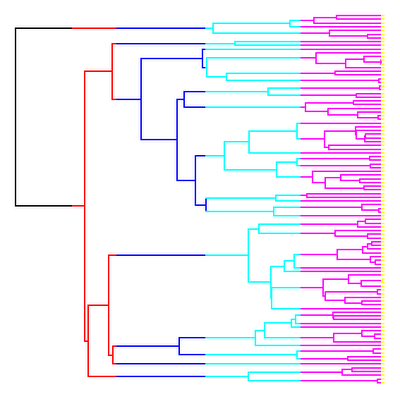
To see the improvement in computation time that is provided by REML in this case, download the source file (here), and try out the following exercise. (Note that on a tree with 1000 terminal species, as in this example, be forewarned that brownie.lite() will take several minutes to run.)

> require(geiger); require(phytools)
> set.seed(10) # for repeatability
> tree<-drop.tip(birthdeath.tree(b=1,d=0,taxa.stop=1001),"1001")
> tree<-rescaleTree(tree,1)
> tree<-sim.history(tree,matrix(c(-1,1,1,-1),2,2))
> x<-sim.rates(tree,c(1,10))
names absent from sig2: assuming same order as $mapped.edge
> system.time(result1<-brownie.lite(tree,x))
   user  system elapsed 
 353.53    3.39  357.70 
> source("brownieREML.R")
> system.time(result2<-brownieREML(tree,x))
   user  system elapsed 
   0.28    0.00    0.28 
> result1
$sig2.single
[1] 6.477488
...
$logL1
[1] -1348.224
...
$sig2.multiple
       1        2 
1.010363 9.819315 
...
$logL.multiple
[1] -1160.006
...
> result2
$sig2.single
[1] 6.483972
$logL1
[1] -1347.577
$sig2.multiple
       1        2 
1.012534 9.824353 
$logL2
[1] -1159.737
$convergence
[1] TRUE

I anticipate that brownieREML() will be added to future versions of the "phytools" library.

phytools manuscript accepted

Quick post - the manuscript describing "phytools" was recently accepted at Methods in Ecology & Evolution. See blog post here.

New version of phyl.RMA() with fixed lambda

I just posted a new version of my R function for phylogenetic reduced major axis regression (RMA), called phyl.RMA(). Since the RMA slope is merely computed as the variance ratio, this function just computes phylogenetic variances and then takes their ratio. The function also (for method="lambda") first performs joint estimation of Pagel's λ (e.g., see Freckleton et al. 2002). Direct link to the code is here.

The new feature of this version of the function (as requested by a user) is merely that the value of λ can be fixed by the user rather than estimated. This is done by calling phyl.RMA(...,fixed=TRUE,lambda=XX). So, for instance, try the following:

> require(geiger)
> require(phytools)
> source("phyl.RMA.R")
> tree<-drop.tip(birthdeath.tree(b=1,d=0,taxa.stop=201),"201")
> X<-fastBM(lambdaTree(tree,0.7),nsim=2)
> phyl.RMA(X[,1],X[,2],tree,method="lambda")
$RMA.beta
[1] -0.0866432 1.0590274
$V
x y
x 0.97406967 -0.03095092
y -0.03095092 1.09245711
$lambda
[1] 0.734092
$logL
[1] -770.6879
$resid
[,1]
21 -5.863653843
101 -5.841695560
...

If we wanted to know, say, if the estimated value of λ (here ~0.73) was significantly different than 0.0 (or any other value), we can fix λ at 0.0 and recalculate:

> phyl.RMA(X[,1],X[,2],tree,method="lambda",fixed=T,lambda=0)
$RMA.beta
[1] -0.7000868 0.9720490

$V
x y
x 0.75527418 -0.09025328
y -0.09025328 0.71364296

$lambda
[1] 0

$logL
[1] -845.7699

$resid
[,1]
21 -5.01116336
101 -4.87370275
...

Cool!

Unfortunately, it has just been reported to me that we have had an escaped anole from the common garden Anolis carolinensis rearing experiment that is presently taking place in my lab. Time to go lizard hunting!

New function to plot "eras" on the tree

I just created and posted a new function, make.era.map(), that maps "eras" (that is, spans of time defined by a set of limits above the root node of the tree) on a phylogeny. Source code is here. To illustrate what I mean by that, let's load the function & try it:

> require(phytools)
Loading required package: phytools
Loading required package: ape
...
> require(geiger)
Loading required package: geiger
...
> setwd("make.era.map/")
> source("make.era.map.R")
> tree<-drop.tip(birthdeath.tree(b=1,d=0,taxa.stop=101),"101")
> tree<-rescaleTree(tree,290)

Now let's define our eras on the tree:

> periods<-c(290,245,210,140,65,1.5)
> names(periods)<-c("P","Tr","J","C","Te","Q")
> periods
    P    Tr    J    C    Te    Q
290.0 245.0 210.0 140.0 65.0 1.5

Now let's use make.era.map() and plotSimmap() to map & plot these geological periods on the tree. Note, that I will plot the limits as 290 minus the limits, because the function normally accepts times from the root node (not from the present, as we have expressed these geological time periods).

> mtree<-make.era.map(tree,290-periods)
> cols<-c(1,2,4:7); names(cols)<-names(periods)
> plotSimmap(mtree,cols,pts=0,ftype="off")

This is what we get:


Pretty cool, huh?

To illustrate the use of this analysis, let's imagine we wanted to test the hypothesis (say, using the approach of O'Meara et al. 2006) that the rate of evolution for a phenotypic trait changed as a function of geological period. The first thing we need to do is plot the geological periods on the tree, as we have done using make.era.map(). Next we fit the model to our mapped tree and the data using brownie.lite()

In this case, since we don't actually have real data - let's simulate some. We can do that using the phytools function sim.rates(). Let's pretend the evolutionary rate declined with each passing era (halving, in this case):

> sig2<-2^(5:0); names(sig2)<-names(periods)
> sig2
P Tr J C Te Q
32 16 8 4 2 1
> X<-sim.rates(mtree,sig2)

Now we can fit the model:

> X<-sim.rates(mtree,sig2)
> fit<-brownie.lite(mtree,X,maxit=4000)
> fit
$sig2.single
[1] 2.975852
...
$logL1
[1] -399.7999
$k1
[1] 2
$sig2.multiple
P Tr J C Te Q
0.002975852 29.886666888 6.587138450 5.385521826 2.102272018 1.078584364
...
$logL.multiple
[1] -393.0759
$k2
[1] 7
$P.chisq
[1] 0.01952338
$convergence
[1] "Optimization has converged."

Note, that there is very little power in the deepest period represented on the tree because this is only covered by two branches!

I will post more on how I did this tomorrow.

Small error in phylosig(), fixed

I realized today after posting the new version of phylosig() online yesterday (described here) that I had made one small error. That is, in the function call the user must assign the variable se, implying "standard errors," but in the function code I treat these as sampling variances (i.e., the square of the SE) rather than as standard errors. This has now been fixed (but please download v0.5 here), so the user can supply a (named) vector of standard errors as intended.

Phylogenetic signal with measurement error

I just posted a new version of the function phylosig() that computes phylogenetic signal using Blomberg's K (Blomberg et al. 2003) and Pagel's λ methods.

The main improvement of this version is that I have added estimation of K with known measurement error, following Ives et al. (2007). This was in response to a user's email request.

This was not too difficult. Basically, without measurement error the values for the tip states on the tree under BM are distributed as a multivariate normal with variance-covariances given by σ²C, where C is an n×n matrix (for n species) containing the height above the root node of the common ancestor of each i,jth species pair on the tree. (For diagonal elements, these are just the heights of each tip node.)

With measurement error, the picture complicates slightly. Now, say the VCV matrix for the measurement error is given by M, then the multivariate distribution of the tip values is given by σ²C+M. The only problem with this is that although we have an analytic solution for σ² conditioned on no measurement error, we do not for known M. Instead, we have to find σ² by other means - say, by maximizing the likelihood. This is what I have done in the latest version of phylosig() (v0.4), available here.

To run this, first download the source and load "phytools":

> require(phytools)
> source("phylosig.R")

Now, just for fun, let's simulate data with measurement error.

> tree<-drop.tip(birthdeath.tree(b=1,d=0,taxa.stop=301),"301")
> x<-fastBM(tree) # simulate data
> se<-rchisq(n=300,df=1) # simulate SEs
> names(se)<-names(x)
> e<-rnorm(n=300,sd=se)
> xe<-x+e

We have data generated without error (in x) and with known error (in xe). First, let's compute phylogenetic signal for x:

> phylosig(tree,x)
[1] 1.013599

This is more or less what we expect. Now let's try xe, but with measurement error ignored:

> phylosig(tree,xe)
[1] 0.2640041

Finally, we can try our new function incorporating measurement error:

> phylosig(tree,xe,se=se)
$K
[1] 1.121445

$sig2
[1] 0.9772118

$logL
[1] -543.0133

Very cool! Note that the logL reported here is the log-likelihood for the value of sig2 conditioned on the known measurement error we've provided.

Of course, this is not magic - so the more measurement error we have, the less power we will have to measure phylogenetic signal. That said, incorporating measurement error has the nice property of making our estimates of signal unbiased (whereas they are biased downwards when signal is ignored).

New version of phytools (v0.1-0) on CRAN

I just submitted a new version of "phytools" to CRAN and it is now available online (phytools CRAN page here). This new version (v0.1-0) has a number of new functions over the previous CRAN version (v0.0-8) but little in terms of functional updates from the last version of "phytools" v0.0-9 which I posted on my website but not to CRAN. Most of the updates in the latest version involve improving the documentation (although there is still a lot of work to be done in this area); removing strictly internally used functions from the namespace (this means they can no longer be accessed by users, which is good); and moving a number of little-used dependencies from "Depends" to "Imports." This helps avoid cluttering the namespace (that is, having too many packages loaded with all their named functions stored in memory).

Note that at time of writing, the Windows & Mac OS versions of "phytools" were still migrating through cyberspace to all the mirror CRAN repositories. Thus, to download the latest version of "phytools" in binary form, please check the list of CRAN mirrors to find one that has the binary versions uploaded (e.g., Austria; please note that in general it is a good idea to pick a CRAN mirror geographically near to you so as to minimize network load).

Comments, problems welcome.