Simulating an irreversible discrete trait using sim.history()

A user asked how one should go about simulating a character that evolves from state "0" (say) to state "1", but not the reverse. This corresponds to the following transition matrix:

> Q
   0 1
0 -1 0
1  1 0

in which we can substitute any instantaneous transition rate for the 1.0 and -1.0. Unfortunately, for various reasons sim.history doesn't work for transition rates of exactly zero - however it works fine if we substitute a value slightly greater than zero. To see this work, try the following example code that uses "geiger" and "phytools":

require(phytools)
require(geiger)
tree<-drop.tip(birthdeath.tree(b=1,d=0,taxa.stop=101),"101")
tree<-rescaleTree(tree,1)
Q<-matrix(c(-1,1,1e-10,-1e-10),2,2)
rownames(Q)<-colnames(Q)<-c("0","1")
mtree<-sim.history(tree,Q,"0")
cols<-c("blue","red"); names(cols)<-c(0,1)
plotSimmap(mtree,cols,ftype="off")

which should produce something that looks like this:



Don't forget, of course, that the tip states are stored in mtree$states, i.e.:

> mtree$states
 53  98  99  24  25  26  18  13  30  31  56  80 
"0" "0" "0" "0" "0" "0" "0" "0" "1" "1" "1" "1" 
 81  77  ...
"1" "1"  ...

phytools version 0.1-2

I just posted a new version of phytools, version 0.1-2, to my webpage, here. I have also submitted this version to CRAN (but it will probably take a day or two to be accepted, and then a few days more to percolate through all the mirror repositories). In the meantime, it can be installed in Windows by downloading the file phytools_0.1-2.zip and then typing:

> install.packages("phytools_0.1-2.zip",repos=NULL)

at the prompt. (For instructions on how to install on Mac/Linux/Unix from source, please see my website.)

New features in this version of phytools include:

1) A new function, anc.Bayes(), for Bayesian ancestral state estimation.

2) A new function, vcvPhylo(), to compute the so-called phylogenetic variance covariance matrix including ancestral nodes. I posted about this function here.

Check it out!

Major speed up of anc.Bayes()

I just realized how to score a major speed-up in computation time from my new Bayesian ancestral character estimation function for continuous traits (anc.Bayes). Last night I documented what I thought at the time was a significant speed improvement. By pulling inversion of the phylogenetic VCV matrix out of the likelihood function (meaning that we only have to do this once instead of every generation of the MCMC), I was able to cut computation time in half (from about 60s on a 100 taxon tree to about 30s). What I didn't realize at the time was that I could also pull out calculation of the determinant of the matrix. The determinant we want is log(|σ²C|); the way we avoid recalculating this every generation of the MCMC (in which σ² can potentially differ) is by taking advantage of the equality:

log(|σ²C|) = nlog(σ²) + log(|C|)

I actually described this in an earlier paper with Luke Harmon (Revell & Harmon 2008, p. 318), but did not think to apply it to this problem until now. [Note that there is actually a small error in equation (5) of our article: n·r·log(k) should be n·r·log(k)/2.]

This version runs much faster: now about 4s for the same dataset as before. Unbelievable! Anyway, I have posted the new version on my website here.

This version is so much faster that I can easily run it for a million generations on the 100 species tree from before. If I plot the estimates from the Bayesian MCMC run with an uninformative prior against the values from ML estimation using ace() in the ape package, we can see that they are even more tightly correlated than before:

> source("anc.Bayes.R")
> source("vcvPhylo.R")
> X<-anc.Bayes(tree,x,ngen=1000000)
> plot(ace(x,tree)$ace,colMeans(X[21:10001,])[2+1:tree$Nnode])


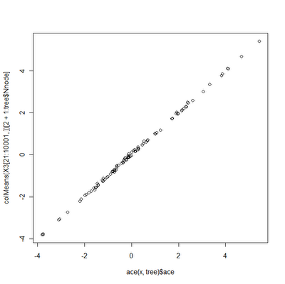
(compare to here). The above code took about 6 minutes to run, whereas the first version of anc.Bayes would've needed about 100 minutes for the same calculations.

I haven't mentioned MCMC diagnostics, priors, or the utility of Bayesian inference at all yet. Hopefully, these will be addressed in future posts.

Improvement to anc.Bayes()

I have already identified a major area in which I can easily improve the computation time of anc.Bayes(), my new function for Bayesian MCMC ancestral state estimation. Specifically, after having thought myself quite clever for using dmnorm() in the mnormt library (see post here), I realized that this was actually extremely computationally inefficient - especially for large matrices. This is because by using dmnorm() I'm essentially forced R to invert our VCV matrix (which is of order number of tips + number of nodes) every generation of the MCMC. This is totally unnecessary and I can easily create a custom function to compute the MVN probability density in which I avoid inverting the phylogenetic VCV matrix on each call. This function is below (it still requires that we invert C once), and I will post a new version of anc.Bayes() tomorrow.

likelihood<-function(C,invC,x,sig2,a,y){
  logLik<--(c(x,y)-a)%*%invC%*%(c(x,y)-a)/(2*sig2) -nrow(invC)*log(2*pi)/2 -determinant(sig2*C,log=T)$modulus[1]/2
  return(logLik)
}

Bayesian ancestral character estimation

I've just been working on a new function for Bayesian ancestral character estimation (anc.Bayes). I'm still working out some of the bugs, but I have nonetheless posted a preliminary version online, here. (It also uses vcvPhylo(), which can be downloaded here).

A couple of comments about doing this.

1) If we take advantage of the multivariate normal density function dmnorm in the mnormt package, and my function vcvPhylo(), computing the likelihood (which we will use to calculate the posterior odds ratio) can be done in just a few lines of code:

C<-vcvPhylo(tree)
# function returns the log-likelihood
likelihood<-function(C,x,sig2,a,y){
  logLik<-dmnorm(x=c(x,y),mean=rep(a,nrow(C)),varcov=sig2*C, log=TRUE)
  return(logLik)
}

in which x is the data for species, y are the ancestral character values, a is the state at the root node, and sig2 is the evolutionary rate.

2. All the control parameters of the Bayesian MCMC (starting values, proposal distributions, and prior probabilities) are accessible to the user - but I have also tried to give the function the capacity to give reasonable values for these things if they are not provided by the user.

Although I'll warn again that this I am still working on this, it is not too soon to try it out. Let's simulate, run the MCMC, and then compare the results to ML estimates obtained using ace() in the ape package:

> require(phytools)
> source("vcvPhylo/vcvPhylo.R")
> source("anc.Bayes/anc.Bayes.R")
> set.seed(100)
> tree<-rtree(100)
> x<-fastBM(tree,sig2=2)
> result<-anc.Bayes(tree,x,ngen=100000)
Control parameters (set by user or default):
List of 7
 $ sig2   : num 2.03
 $ a      : num [1, 1] 0.00737
 $ y      : num [1:98] 0.00737 0.00737 0.00737 0.00737 0.00737 ...
 $ pr.mean: num [1:100] 1000 0 0 0 0 0 0 0 0 0 ...
 $ pr.var : num [1:100] 1e+06 1e+03 1e+03 1e+03 1e+03 1e+03 1e+03 1e+03 1e+03 1e+03 ...
 $ prop   : num [1:100] 0.142 0.142 0.142 0.142 0.142 ...
 $ sample : num 100
Starting MCMC...
Done MCMC.
> # plot the result against the MLEs
> plot(ace(x,tree)$ace,colMeans(result[21:1001,])[2+1:tree$Nnode])

Here, we get the following result:


Obviously, I will post more on this as I improve it and I will also try to provide more guidance on MCMC control and priors.

Faster vcvPhylo() with ancestral nodes

In my last post I put up a simple version vcv.phylo() (which returns a matrix containing the height above the root of each pair of species in the tree, sometimes called the phylogenetic variance-covariance matrix), but that included ancestral nodes. I pulled this out of an old function of mine, anc.trend(), so I figured I could do better - and after some tinkering I came up with a much improved version, as follows:

vcvPhylo2<-function(tree,anc.nodes=T){
  n<-length(tree$tip.label)
  h<-nodeHeights(tree)[order(tree$edge[,2]),2]
  h<-c(h[1:n],0,h[(n+1):length(h)])
  M<-mrca(tree,full=anc.nodes)[c(1:n,anc.nodes*(n+2:tree$Nnode)),c(1:n,anc.nodes*(n+2:tree$Nnode))]
  C<-matrix(h[M],nrow(M),ncol(M))
  if(anc.nodes) rownames(C)<-colnames(C)<-c(tree$tip.label,n+2:tree$Nnode)
  else rownames(C)<-colnames(C)<-tree$tip.label
  return(C)
}

A couple of tricks in here:

1) Rather than calling dist.nodes(), this function uses the phytools function nodeHeights, which returns a matrix of the dimensions of tree$edge, containing the height above the root of every node, and is quite fast.

2) The function then uses mrca(...,full=T) in the ape package, which returns the MRCA of every pair of species and nodes. This essentially serves as an index to construct our VCV matrix from the node heights!

All of this is done with the following lines of code:

# this gets a vector of height by node number
h<-nodeHeights(tree)[order(tree$edge[,2]),2]
# this inserts a height of zero for the root node (node n+1 for n species)
h<-c(h[1:n],0,h[(n+1):length(h)])
# this is our index matrix
M<-mrca(tree,full=T)
# this is our VCV matrix
C<-matrix(h[M],nrow(M),ncol(M))

Let's compare computation time to vcv.phylo and our earlier version (vcvPhylo1):

> tree<-rtree(500)
> system.time(X<-vcv.phylo(tree)) # only tips
   user  system elapsed 
   2.20    0.00    2.22 
> system.time(Y<-vcvPhylo1(tree)) # tips & nodes, old version
   user  system elapsed 
   7.68    0.03    7.73 
> system.time(Z<-vcvPhylo2(tree)) # tips & nodes, new version
   user  system elapsed 
   3.49    0.05    3.54 
> all(Y==Z)
[1] TRUE
> all(X==Z[c(1:500),c(1:500)])
[1] TRUE

Cool! BTW - Happy Thanksgiving to all the blog readers.

vcv.phylo() with ancestral nodes

An R-sig-phylo user just posted a request for a function to compute the so-called phylogenetic variance-covariance matrix. That is, the N×N matrix (for N species) containing in position i,j the height above the root of the MRCA of species i and j (as done in the ape function vcv.phylo) - but including ancestral nodes. As it turns out, I have a code fragment to do this in my function anc.trend() (link here). I pasted the fragment into a function vcvPhylo() as follows:

vcvPhylo<-function(phy,anc.nodes=T){
  if(anc.nodes){
    D<-dist.nodes(phy)
    ntips<-length(phy$tip.label)
    Cii<-D[ntips+1,]
    C<-D; C[,]<-0
    for(i in 1:nrow(D)) for(j in 1:ncol(D)) 
      C[i,j]<-(Cii[i]+Cii[j]-D[i,j])/2
    dimnames(C)[[1]][1:length(phy$tip)]<-dimnames(C)[[2]][1:length(phy$tip)]<-phy$tip.label
    C<-C[c(1:ntips,(ntips+2):nrow(C)),c(1:ntips,(ntips+2):ncol(C))]
    return(C)
  } else return(vcv.phylo(phy))
}

and it seems to do the trick.