New version of plotSimmap that can plot node numbers

I just posted a new version of plotSimmap (direct link to code here) which can also plot node numbers (that is, the numbers in the matrix $edge for all non-terminal nodes). These are the same labels used by nodelabels in ape if no node names have been assigned.

This was pretty easy. I just plotted a rectangle with white background (using the graphics function symbols) at the end of each branch not ending in a tip. (I have to figure out where these branches go anyway, so the problem of identifying the vertical position is already solved.) I specified the height & width of box to be slightly larger than the label text length & width using strheight and strwidth. I then wrote inside the box using text.

The result can be visualized by doing something like the following:

require(phytools)
source("plotSimmap.R") # load the new version of plotSimmap
Q<-matrix(c(-1,1,1,-1),2,2)
cols<-c("blue","red"); names(cols)<-c(1,2)
tree<-sim.history(pbtree(n=25,scale=1),Q,anc=1)
plotSimmap(tree,cols,lwd=3,pts=F,node.numbers=T)



That's pretty cool. Since plotTree is now just a wrapper for plotSimmap with a really simple change to plotTree (code here) you can now visualize node numbers using that function as well (although this is pretty much completely redundant with plot.phylo and nodelabels in ape).

source("plotTree.R") # load the new version of plotTree
plotTree(tree,pts=F,lwd=3,node.numbers=T)



That's it!

Ottawa SSB symposium

The speaker line-up for the SSB symposium I am co-organizing with Cécile Ané has been posted online on the Evolution 2012 website here.

Here are the details (with added links to speaker websites):

New phylogenetic methods for quantitative trait evolution

Organizers: Cécile Ané (University of Wisconsin-Madison) and Liam J. Revell (University of Massachusetts Boston)

Speakers:
   · Cécile Ané (University of Wisconsin)
   · Carl Boettiger (University of California, Davis)
   · Joseph Felsenstein (University of Washington)
   · Brian C. O'Meara (University of Tennessee)
   · Liam J. Revell (University of Massachusetts)
   · Lars Schmitz (University of California, Davis)

Should be fun!

New function to paint sub-trees with different states

I just posted a new function to "paint" subtrees on a phylogeny with different mapped states. I did this in response to a user request and the purpose is to allow users to specify arbitrary mapping for use in functions like brownie.lite, brownieREML, and evol.vcv. The name of this new function is paintSubTree and a direct link to the function code is here.

The way this function works is pretty straightforward. Basically, it takes the tree & the basal node number of a sub-tree on the phylogeny. It then paints all the tipward edges of that node (as well as the stem, if selected) in an arbitrarily specified state. Since the function also retains any existing mapping, it can be used multiple times to paint different clades, and even nested clades, in different states.

I accomplished this by first using a function called getDescendants (basically the same as phangorn:Descendants) to compute all the descendant node and tip numbers from the target node. Then I use this set of node numbers (and the handy base function which) to match the tipward nodes to the $edge matrix and then paint the branches accordingly.

Here is a quick illustration of use. First, let's simulate a small tree, set the tip & tip numbers equal, and then plot the tree with node numbers:

> require(phytools)
> tree<-pbtree(n=15); tree$tip.label<-1:15
> plot(tree,font=1); nodelabels(bg="white")



Now let's paint all the edges from node 20 in a derived state, including the stem leading to node 20:

> tree<-paintSubTree(tree,node=20,state="2",stem=T)
> cols<-c("blue","red","green"); names(cols)<-c(1,2,3)
> plotSimmap(tree,cols,lwd=3,pts=F)



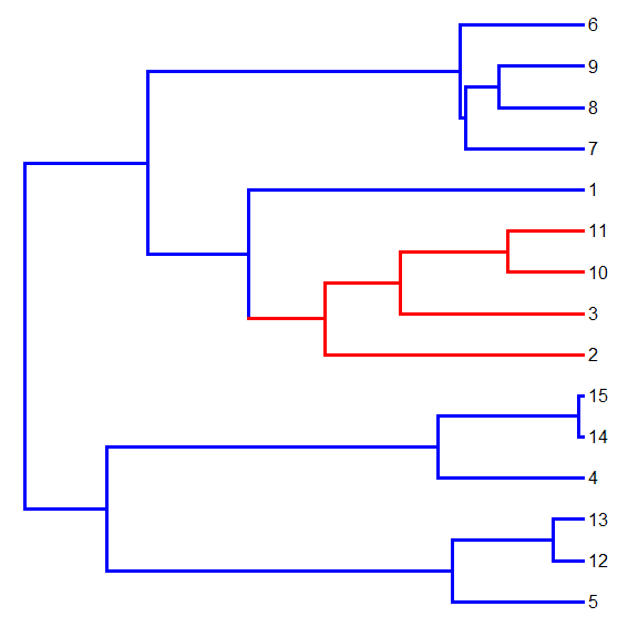
Mission accomplished. Now, let's paint a separate part of the tree, say the clade descending from node 24 (this time excluding the stem), with state 3:

> tree<-paintSubTree(tree,node=24,state="3",stem=F)
> plotSimmap(tree,cols,lwd=3,pts=F)



Finally, we can also paint nested clades as well as only tip edges. If we paint a tip edge only, obviously stem must be set to TRUE. Let's do that:

> tree<-paintSubTree(tree,node=3,state="3",stem=T)
> plotSimmap(tree,cols,lwd=3,pts=F)



Cool.

Function to get descendant node numbers

So, I'm working on a different project that required me to write a function to pull out the descendant node (& tip) numbers from any internal node on the tree. Even though I feel like I've done this before, I struggled coming up with something that made sense. This is what I ended up with:

getDescendants<-function(tree,node,curr=NULL){
  if(is.null(curr)) curr<-vector()
  daughters<-tree$edge[which(tree$edge[,1]==node),2]
  curr<-c(curr,daughters)
  w<-which(daughters>=length(tree$tip))
  if(length(w)>0) for(i in 1:length(w))
    curr<-getDescendants(tree,daughters[w[i]],curr)
  return(curr)
}

Here's a quick example of how it works:

> tree<-pbtree(n=10)
> tree$tip.label<-1:10
> # this lines up tip numbers & labels for simplicity
> par(mar=c(1,1,1,1)) # set margins
> plot(tree,font=1); nodelabels(bg="white")


Now we can pull the numbers for the descendant nodes & tips for any internal node. For instance:

> getDescendants(tree,node=17)
[1] 18 6 7 8
> getDescendants(tree,node=12)
[1] 16 15 4 5 2 3
> getDescendants(tree,node=19)
[1] 9 10

Anyway, seems to work, but if anyone is aware of an existing function for this, please pass it along.

Getting tip states from sim.history

A user just emailed me to ask how you get the tip states from a character history simulated using sim.history. This is pretty easy because sim.history stores them in the vector $states.

So, for one tree:

> require(phytools)
> tree<-pbtree(n=25,scale=1)
> Q<-matrix(c(-1,1,1,-1),2,2)
> mtree<-sim.history(tree,Q)
> mtree$states
t1  t2  t3  t4  t5  t6  t7  t8  t9 t10 t11 t12 t13 t14 t15 t16
"2" "1" "2" "2" "2" "2" "2" "1" "2" "2" "2" "2" "2" "2" "1" "2"
t17 t18 t19 t20 t21 t22 t23 t24 t25
"2" "2" "2" "1" "2" "2" "2" "2" "2"

Or, for multiple trees:

> mtrees<-sim.history(tree,Q,nsim=10)
> mtrees[[1]]$states # first simulated history
t1  t2  t3  t4  t5  t6  t7  t8  t9 t10 t11 t12 t13 t14 t15 t16
"1" "2" "1" "2" "2" "2" "2" "2" "1" "1" "2" "1" "1" "1" "1" "1"
t17 t18 t19 t20 t21 t22 t23 t24 t25
"1" "1" "1" "1" "2" "1" "1" "1" "1"
> mtrees[[2]]$states # second history
t1  t2  t3  t4  t5  t6  t7  t8  t9 t10 t11 t12 t13 t14 t15 t16
"2" "1" "1" "2" "2" "2" "1" "1" "1" "2" "1" "1" "1" "2" "2" "2"
t17 t18 t19 t20 t21 t22 t23 t24 t25
"1" "1" "1" "2" "1" "1" "1" "1" "1"
> # etc, or to get all states from all simulated histories (in columns)
> X<-sapply(mtrees,function(x) x$states) # all histories
> X
    [,1] [,2] [,3] [,4] [,5] [,6] [,7] [,8] [,9] [,10]
t1  "1"  "2"  "2"  "1"  "2"  "1"  "2"  "1"  "1"  "2"  
t2  "2"  "1"  "1"  "2"  "2"  "2"  "1"  "1"  "2"  "2"  
t3  "1"  "1"  "2"  "2"  "1"  "1"  "2"  "2"  "2"  "1"
...

That's it!

Phytools demo vignette

I'm down in Puerto Rico on a lab field trip right now, but while in flight I prepared my recent mini-workshop on phytools that I gave at UCLA in the format of an R vignette. Keep in mind that this demo highlights only a small subset of the capabilities of the phytools package. I have also posted the file to scribd and you can view the embedded PDF below:

Phytools Demo

I apologize that this is a little rough around the edges, but it is my first R vignette and evidently some of the workshop attendees were interested in getting my notes so I wanted to post these as quickly as possible.

Fitting Pagel's λ for a single trait using multiple methods

Because it related to something else I was working on, I today did a quick comparison of the (at least 4) different methods available in R to fit Pagel's λ model for a single trait. I just did this for a single 200 taxon tree and compared the estimates (which are all, to reasonable numerical precision, the same) and the computation time. A more thorough comparison would require that we run this code over multiple simulations to try and determine the robustness of each function. This I have not done, but anyone wishing to loop the following analyses 100 or more times should be my guest. This was run on my VAIO AMD E-450 laptop @ 1.65 GHz (so, not very fast):

> require(phytools); require(geiger); require(caper); require(nlme)
> tree<-pbtree(n=200,scale=1) # simulate tree
> x<-fastBM(lambdaTree(tree,0.7)) # simulate data
> # fit using phytools:phylosig
> system.time(m1<-phylosig(tree,x,method="lambda"))
   user  system elapsed
   2.79    0.00    2.79
> # fit using geiger:fitContinuous
> system.time(m2<-fitContinuous(tree,x,model="lambda"))
Fitting  lambda model:
   user  system elapsed
137.11    0.42  138.90
> # fit using nlme:gls
> d<-data.frame(x)
> system.time(m3<-gls(x~1,data=d,correlation=corPagel(0.5,tree,fixed=F), method="ML"))
   user  system elapsed
  51.56    0.22   53.86
> # fit using caper:pgls
> d<-data.frame(x,names(x)); colnames(d)[2]<-"Species"
> system.time(m4<-pgls(x~1,comparative.data(tree,d,"Species"), lambda="ML"))
   user  system elapsed
  38.13    0.01   38.25

We can then get a summary as follows:

> result<-matrix(c(m1$lambda,m1$logL,
m2$Trait1$lambda,m2$Trait1$lnl,
m3$modelStruct$corStruct[1],m3$logLik,
m4$param["lambda"],m4$model$log.lik),4,2,
dimnames=list(c("phylosig","fitContinuous","gls","pgls"),
c("lambda","logL")),byrow=T)
> result
                 lambda      logL
phylosig      0.7478915 -230.7348
fitContinuous 0.7478919 -230.7348
gls           0.7478922 -230.7348
pgls          0.7478922 -230.7348

So, at least for this example, phylosig is quite a bit faster, but it makes no discernible difference in the results. Why this would be the case is not at all clear to me (phylosig uses the built in optimizer, optimize, and performs full ML not REML), but I hope that it does not come at the cost of robust estimation. Certainly this could be assessed by repeating the above analysis for many simulations.