Three more functions & some more methods in Rphylip

I just added a few more functions to the Rphylip project, my R interface for the PHYLIP package. The new interface functions are Rpars (for PARS), Rmix (for MIX), and Rpenny (for PENNY). All three of these are parsimony method programs: the first does heuristic MP search from unordered, multistate data; whereas the latter do (Wagner, Camin-Sokal, or mixed method) MP searching using heuristic or branch-and-bound algorithms, respectively. More details on the programs can be found by referring to the PHYLIP documentation pages linked above.

I also created a new class of data object, "phylip.data", which just generalizes "proseq" (in Rphylip) and "DNAbin" (in ape), and is very simple.

Here's a quick demo using Rpenny. Note that branch-and-bound should generally not be used for more than a dozen or so taxa (it will become computationally prohibitive quickly).

> require(Rphylip)
Loading required package: Rphylip
Loading required package: ape
> packageVersion("Rphylip")
[1] ‘0.1.14’
> data(primates.bin)
> primates.bin
12 character value sequences stored in a matrix.

All sequences of same length: 231

Labels: Lemur Tarsier Sq.Monkey J.Macaque R.Macaque E.Macaque ...

Trait value composition:
    0     1
0.406 0.594
> tree<-Rpenny(primates.bin)

....

How many
trees looked                                 Approximate
at so far    Length of      How many         percentage
(multiples   shortest tree  trees this long  searched
of  100):    found so far   found so far     so far
----------   ------------   ------------     ------------
     1       -                      0            0.00
     2       -                      0            0.00
     3       -                      0            0.00
     4       208.00000              3            0.00
     5       208.00000              6            0.00
     6       208.00000              6            0.14
     7       208.00000              6            1.90
     8       208.00000              6            6.67
     9       208.00000              6            9.33
    10       208.00000              6           14.00
    11       208.00000              6           37.78
    12       208.00000              6           53.33

Output written to file "outfile"

Trees also written onto file "outtree"

Press enter to quit.

Penny algorithm, version 3.695
 branch-and-bound to find all most parsimonious trees

Wagner parsimony method


                                    requires a total of            208.000

    6 trees in all found


  +--------------------------------1
  ! 
  !  +-----------------------------2        
  !  ! 
--1  !                       +-----10       
  !  !                    +-10 
  !  !                    !  !  +--11       
  !  !                 +--6  +--8 
  !  !                 !  !     +--12       
  +--2     +-----------5  ! 
     !     !           !  +--------9        
     !     !           ! 
     !     !           +-----------8        
     !  +--4 
     !  !  !                 +-----6        
     !  !  !              +-11 
     !  !  !              !  !  +--5        
     +--3  +--------------7  +--9 
        !                 !     +--7        
        !                 ! 
        !                 +--------4        
        ! 
        +--------------------------3        

  remember: this is an unrooted tree!

....

Translation table
-----------------
        1       Lemur
        2       Tarsier
        3       Sq.Monkey
        4       J.Macaque
        5       R.Macaque
        6       E.Macaque
        7       B.Macaque
        8       Gibbon
        9       Orangutan
        10      Gorilla
        11      Chimp
        12      Human

Rooted tree(s) with the outgroup
------------------------
Tarsier, Lemur

> require(phytools)
Loading required package: phytools
Loading required package: maps
Loading required package: rgl
> par(mfrow=c(3,2))
> plotTree(tree)
Waiting to confirm page change...

(These are the six equally most parsimonious trees found by PENNY.)

Cool. The latest version of Rphylip can be downloaded here, and is also on GitHub.

More updates to rateshift method: Testing for the presence of a rate shift

I have made some updates to the function rateshift (first described here) to facilitate comparison of alternative models for rate shifts; as well as for testing the null hypothesis of no shift.

First, I fixed the function so it could fit a no-rate-shift model. That was broken in the previous version, but should work now. When we fit the nrates=1 model, the fitted model parameter value (σ²) and log-likelihood should be the same as from (say) fitContinuous in geiger or the one-rate model in brownie.lite.

Second, I created an S3 generic logLik method for the object of class "rateshift" returned by the function. This allows us to easily extract the log-likelihood & model parameterization; but it also allows us to use the generic AIC to compute the Akaike Information Criterion value for the fitted model.

Finally, third, I fixed a minor bug which sometimes created an incompatibility in the tolerance (basically, the very small values we need to add or subtract from some quantities to make sure that the function does not attempt to evaluate the likelihood where it isn't defined) are inconsistent between rateshift and make.era.map, which is used internally. This required changes to both functions, so the wisest thing to do to get this update is to update phytools to the latest non-CRAN version.

OK. Here's a demo:

> require(phytools)
Loading required package: phytools
Loading required package: ape
Loading required package: maps
Loading required package: rgl
> packageVersion("phytools")
[1] ‘0.3.86’
> ## simulate tree & data
> tree<-pbtree(n=100,scale=1)
> tree<-make.era.map(tree,c(0,0.5,0.8))
> x<-sim.rates(tree,c(1,10,1),internal=TRUE)
names absent from sig2: assuming same order as $mapped.edge
> ## here's a visual of our simulation
> phenogram(tree,x,ftype="off")

> ## peel off ancestral states
> x<-x[tree$tip.label]
>
> ## fit 1 rate model
> fit1<-rateshift(tree,x,nrates=1)
> fit1
ML 1-rate model:
      s^2(1)  se(1)  k  logL   
value 1.7966  0.2542 2  -81.8257

This is a one-rate model.

R thinks it has found the ML solution.

> ## fit 2 rate model
> fit2<-rateshift(tree,x,nrates=2)
> fit2
ML 2-rate model:
      s^2(1)  se(1)  s^2(2)  se(2)  k  logL   
value 6.6364  2.1013  0.785  0.1345 4  -64.3827

Shift point(s) between regimes (height above root):
        1|2    se(1|2)
value  0.806  0.02

R thinks it has found the ML solution.

> ## test 2 rates vs 1 rate
> P2vs1<-as.numeric(pchisq(2*(logLik(fit2)-logLik(fit1)),   df=attr(logLik(fit2),"df")-attr(logLik(fit1),"df"),   lower.tail=FALSE)) > P2vs1
[1] 2.658128e-08
> ## fit 3 rate model
> fit3<-rateshift(tree,x,nrates=3)
> fit3
ML 3-rate model:
      s^2(1)  se(1) s^2(2) se(2)  s^2(3)  se(3)  k  logL
value 1.7181  NaN  6.2815 1.8016  0.7716  0.1345 6  -64.017

Shift point(s) between regimes (height above root):
        1|2    se(1|2) 2|3    se(2|3)
value  0.3058  0.0265  0.8193  0.0141

R thinks it has found the ML solution.

> ## test 3 rates vs 2 rates
> P3vs2<-as.numeric(pchisq(2*(logLik(fit3)-logLik(fit2)),
  df=attr(logLik(fit3),"df")-attr(logLik(fit2),"df"),
  lower.tail=FALSE))
> P3vs2
[1] 0.6934852

This shows us that although the fitted shift points in our third fitted model are fairly close to the gnerating shift points, the fit isn't significantly better than our two rate model. I suspect that, in general, it will probably be easier to find shift points that are closer to the tips of the tree, where there tends to be more edges.

Cool.

New method to locate one or multiple rate shifts on a tree using likelihood

I just posted a new phytools function, rateshift, that fits a model in which there are one or multiple Brownian rate shifts in the tree at different heights above the root. The idea is that we don't need to specify the locations of the rate shifts a priori (as we can already do using brownie.lite); rather, we let the data determine where the rate shifts are located. Turns out that this isn't too hard, it just requires p-1 additional parameters for each extra rate above the root.

It also occurred to me that it's entirely possible this method is already in the literature - in which case, please accept my apologies for having missed it!

In the simplest case, this would just be a model with two evolutionary rates: σ²(1) rootward of the shift, and σ²(2) tipward; and one rate shift. We then jointly maximize the likelihood of the rates & position of the rate shift.

Here's a quick demo:

> require(phytools)
Loading required package: phytools
Loading required package: ape
Loading required package: maps
Loading required package: rgl
> packageVersion("phytools")
[1] ‘0.3.85’
> tree<-pbtree(n=100,scale=1)
> tree<-make.era.map(tree,c(0,0.5,0.8))
> x<-sim.rates(tree,c(1,10,1))
names absent from sig2: assuming same order as $mapped.edge
> fit<-rateshift(tree,x,nrates=3,print=TRUE,plot=TRUE, tol=1e-5)
Optimization progress:

s^2(1)  s^2(2)  s^2(3)  shift:1 shift:2 logL
2.623   2.623   2.623   0.3333  0.6667  -117.6615
2.624   2.623   2.623   0.3333  0.6667  -117.6616
....

2.1182  7.6728  0.7129  0.5497  0.8235  -100.7116
2.1182  7.6728  0.7109  0.5497  0.8235  -100.7163
2.1182  7.6728  0.7119  0.5507  0.8235  -100.7079
....
1.1796  8.6499  0.7848  0.5886  0.8116  -100.1251
1.1796  8.6499  0.7848  0.5896  0.8126  -100.1175
1.1796  8.6499  0.7848  0.5896  0.8106  -100.1275

> fit
ML 3-rate model:
      s^2(1) se(1)  s^2(2) se(2)  s^2(3) se(3)  k  logL
value 1.1796 0.991  8.6499 2.3647 0.7848 0.1709 6  -100.12

Shift point(s) between regimes (height above root):
        1|2     se(1|2) 2|3     se(2|3)
value   0.5896  0.0173  0.8126  0.0173

R thinks it has found the ML solution.

The options plot & print slow down runtime; however I included them for the purposes of debugging and it is kind of neat to visualize the optimization of the locations of the rate shift.

The implementation is a little buggy - however at least in this example it seems to do pretty well at finding our generating rate shift points (which were, remember, 0.5 & 0.8 units above the root), and rates (1, 10, & 1). Cool!

This function is in a new phytools build (phytools 0.3-85), which can be downloaded & installed from source. Please check it out.

Three years of blogging

It's now been three years since I starting blogging about phylogeny methods on blog.phytools.org (originally phytools.blogspot.com) - and so, in the tradition of 2011 and 2012, I thought I'd spend a few minutes talking about what I did this year in the phytools package and on the blog.

According to the (somewhat dubious, in my opinion) blogger.com page stats, the phytools blog received upwards of 150,000 page views in 2013. Even if 1/2 of these were by bots, that is still quite an impressive tally. Certainly, by any measure the popularity of the phytools blog as a free repository of information about phytools and phylogeny methods has increased over the past year.

Towards the end of 2012 and throughout 2013 I added considerably to the plotting capabilities of phytools (evidenced, in part, by my recent MEE paper on some new plotting methods). Consequently, it's no great surprise that two of the most viewed phytools blog posts of 2013 included the description of a new method to visualize uncertainty on a traitgram, and some of the description and illustration of the new plotting functions contMap and densityMap, including this description of a published use of both methods in the same figure (which probably didn't hurt by having been re-tweeted by @systbiol). Nestled also among the top three most popular blog posts of 2013 was this comment on why we don't normally expect the residuals from phylogenetic ANOVA or regression to be normally distributed. Also popular were a wide range of posts about stochastic mapping and ancestral state reconstruction, including information about a new method based on the the threshold model from evolutionary quantitative genetics.

Towards the end of 2013, I started on a new project Rhylip. The purpose of Rphylip is to create an R interface for all 30+ programs in the PHYLIP phylogeny method software package by Joe Felsenstein. This will hopefully allow the many functions of PHYLIP to be used seamlessly within an integrated R workflow. (Here's an example of Rphylip at work - created for my phylogeny methods class using knitr.) I'm about 50% of the way there, so I hope to get this done soon.

Finally, I recently learned that my CAREER proposal to do phylogeny method research in several new areas has been recommended for funding by the NSF DEB Systematic Biology program. (Prospective students & postdocs take notice - I will be hiring in 2014!) This comes exactly at the right time as my start-up is in its dying breaths right now. Interestingly, part of the original ulterior motive in developing this blog back towards the end of 2010 was as a supporting 'broader impact' for what was at that time my first attempt to acquire funding for phylogeny method research from the NSF. Thus, the NSF is in part responsible for this blog & phytools as a community resource even without having funded it! (Until now, that is.)

Happy 2014 & thanks for reading!

S3 print method for brownie.lite

Today I wrote an S3 print method for objects returned by the phytools function brownie.lite. This function implements the method of O'Meara et al. (2006) in which we fit different rates of evolution to different parts of a phylogeny (sometimes, say, determined by a mapped discrete character). Print methods are nice because they allow us to tell R how to summarize the content of a complicated object, like a phylogeny or the results of numerical optimization.

The object returned by brownie.lite is unchanged, except that it is now assigned the class attribute "brownie.lite". Here's how it works:

> require(phytools)
> packageVersion("phytools")
[1] ‘0.3.83’
> ## first let's simulate some data
> Q<-matrix(c(-1,1,1,-1),2,2)
> rownames(Q)<-colnames(Q)<-letters[1:2]
> tree<-sim.history(pbtree(n=100,scale=1),Q,anc="a")
> ## simulate with a rate difference among states
> x<-sim.rates(tree,setNames(c(1,2),letters[1:2]))
> ## simulate without a rate difference
> y<-fastBM(tree)
> plotSimmap(tree,setNames(c("blue","red"),letters[1:2]), lwd=3,ftype="off")

> fitx<-brownie.lite(tree,x)
> fitx # this is the same as print(fitx)
ML single-rate model:
          s^2     se      a       k  logL
parameter 1.5484  0.2191  -0.4682 2  -73.73

ML multi-rate model:
          s^2(a)  se(a)   s^2(b)  se(b)   a       k  logL
parameter 0.732   0.2243  1.8163  0.2955  -0.499  3  -70.93

P-value (based on X^2): 0.0179

R thinks it has found the ML solution.

> fity<-brownie.lite(tree,y)
> fity
ML single-rate model:
          s^2     se      a       k  logL
parameter 1.0646  0.1507  -0.7218 2  -55.00
      
ML multi-rate model:
          s^2(a)  se(a)   s^2(b)  se(b)   a       k  logL
parameter 0.8925  0.2661  1.1209  0.1841  -0.7271 3  -54.79

P-value (based on X^2): 0.5184

R thinks it has found the ML solution.

This version of phytools can be downloaded here and installed from source.

More functions & fixes in Rphylip

My latest updates to Rphylip, an R interface for Felsenstein's phylogeny methods package PHYLIP, includes Rdnainvar, an interface for dnainvar, a program for Lake's invariants from DNA sequences; and Rfitch, an interface for fitch, a program that does least-squares and minimum evolution phylogeny inference.

In addition to this, though, today I added the functions setPath & clearPath. The former can be used to set the path to the PHYLIP executables folder for the current R session. Normally, Rphylip tries to find the path to the PHYLIP executable using the internal Rphylip function, findPath. However this function only works if the PHYLIP folder is in a sensible location, such as in C:/Program Files/ (for Windows) or /Applications/ (for Mac OS). If not, the path can always be supplied to the function directly. What setPath does is enable the user to set a different place to look for PHYLIP executables for the current R session. It does this by setting the environmental variable "phylip.path". clearPath does the opposite. It removes the environmental variable "phylip.path" thus permitting Rphylip functions to search for PHYLIP executables in the regular places.

Here's a demo in which I have PHYLIP installed in C:/Users/Liam/Documents/Phylogeny_Programs/:

> require(Rphylip)
Loading required package: Rphylip
Loading required package: ape
> packageVersion("Rphylip")
[1] ‘0.1.13’
> data(primates)
> D<-Rdnadist(primates)
Error in Rdnadist(primates) :
  No path provided and was not able to find path to dnadist
> setPath("C:/Users/Liam/Documents/Phylogeny_Programs/phylip-3.695/exe/")
> D<-Rdnadist(primates)

...

Nucleic acid sequence Distance Matrix program, version 3.695

...

> tree<-Rfitch(D)

...

Fitch-Margoliash method version 3.695

...

  12 Populations

Fitch-Margoliash method version 3.695

                  __ __             2
                  \  \   (Obs - Exp)
Sum of squares =  /_ /_  ------------
                                2
                   i  j      Obs

Negative branch lengths not allowed

global optimization


                                         +-----------7
                                +--------2
                                !        !   +-------6
                                !        +---1
                                !            !  +-4
                       +--------3            +--8
                       !        !               +----5
                       !        !
                       !        !      +-----------------8
                       !        +------9
                       !               !   +-------------9
  +--------------------7               +---5
  !                    !                   !    +-------10
  !                    !                   +----6
  !                    !                        ! +------12
  !                    !                        +-4
  !                    !                          +-------11
  !                    !
  !                    +----------------------------3        
  ! 
 10--------------------------------------2
  ! 
  +-------------------------------------1


remember: this is an unrooted tree!

Sum of squares =     0.68048

Average percent standard deviation =     7.23497

...

Translation table
-----------------
        1       Lemur
        2       Tarsier
        3       Sq.Monkey
        4       J.Macaque
        5       R.Macaque
        6       E.Macaque
        7       B.Macaque
        8       Gibbon
        9       Orangutan
        10      Gorilla
        11      Chimp
        12      Human

> plot(tree)

New di2multi function for stochastically mapped trees

I just posted some code the collapses internal branches of zero length (or, more specifically, branches with length shorter than some arbitrarily specified value tol) to polytomies for trees with mapped discrete characters created using (for instance) make.simmap or read.simmap. This is exactly the same as di2multi in the ape package (functionally - I programmed it totally differently, hopefully not at the peril of users); however it works for modified "phylo" objects with a mapped discrete trait.

The code to the function is here, but it uses internal phytools functions - so for it to work, you will probably have to install the latest version of phytools (here).

Here's a quick demo of the function at work:

> require(phytools)
> packageVersion("phytools")
[1] ‘0.3.81’
> ## first create a tree with some polytomies
> N<-26
> tree<-pbtree(n=N,tip.label=LETTERS[26:1],scale=1)
> tree$edge.length[tree$edge.length<0.1&tree$edge[,2]>N]<-0
> ## make the tree ultrametric
> d<-max(vcv(tree))-diag(vcv(tree))
> tree$edge.length[tree$edge[,2]<=N]<- tree$edge.length[tree$edge[,2]<=N]+d
> ## check is ultrametric
> is.ultrametric(tree)
[1] TRUE
> ## check is binary
> is.binary.tree(tree
[1] TRUE
> ## simulate discrete character history on tree
> Q<-2*matrix(c(-1,1,1,-1),2,2)
> tree<-sim.history(tree,Q)
> plotSimmap(tree,colors=setNames(c("blue","red"),1:2), lwd=3)

> ## collapse branches of zero length
> tree<-di2multi.simmap(tree)
> ## check is binary
> is.binary.tree(tree)
[1] FALSE
> plotSimmap(tree,colors=setNames(c("blue","red"),1:2), lwd=3)

The main reason this might be important is because densityMap runs into problems when your tree has internal edges that are very short. This can be addressed by first collapsing all zero/small branches in each of the stochastic mapped trees, and then computing the density-map on the collapses stochastic mapped trees. Code for that would look like the following:

trees<-lapply(trees,di2multi.simmap)
class(trees)<-"multiPhylo"
densityMap(trees)

Three different ways to calculate the among-species variance-covariance matrix for multiple traits on a phylogeny

Here are three different ways to compute the among-species variance-covariance matrix for multiple characters on the tree. If we assume that the characters are evolving by Brownian motion, this matrix is an unbiased estimate of the instantaneous diffusion matrix of the evolutionary process.

The three options are (1) the GLS estimating equation (used in Revell 2009); (2) the method of equation 5 in Butler et al. (2000); and (3) we can use PICs (Felsenstein 1985).

Here is code to do each of these in R:

## compute evolutionary VCV matrix using method of
## Revell (2009)
A<-matrix(1,nrow(X),1)%*%apply(X,2,fastAnc,tree=tree)[1,]
V1<-t(X-A)%*%solve(vcv(tree))%*%(X-A)/(nrow(X)-1)

## compute evolutionary VCV matrix using method of
## Butler et al. (2000)
Z<-solve(t(chol(vcv(tree))))%*%(X-A)
V2<-t(Z)%*%Z/(nrow(X)-1)

## compute the evolutionary VCV matrix using pics
Y<-apply(X,2,pic,phy=tree)
V3<-t(Y)%*%Y/nrow(Y)

OK - now let's try it with some simulated data:

> ## load packages
> require(phytools)
Loading required package: phytools
Loading required package: ape
Loading required package: maps
Loading required package: rgl
> ## simulate tree & data
> simV<-matrix(c(1,1.2,0,1.2,2,0,0,0,3),3,3)
> simV ## generating covariance matrix
     [,1] [,2] [,3]
[1,]  1.0  1.2    0
[2,]  1.2  2.0    0
[3,]  0.0  0.0    3
> tree<-pbtree(n=100,scale=1) ## simulate tree
> X<-sim.corrs(tree,simV) ## simulate data
>
> ## Revell (2009)
> A<-matrix(1,nrow(X),1)%*%apply(X,2,fastAnc,tree=tree)[1,]
> V1<-t(X-A)%*%solve(vcv(tree))%*%(X-A)/(nrow(X)-1)
>
> ## Butler et al. (2000)
> Z<-solve(t(chol(vcv(tree))))%*%(X-A)
> V2<-t(Z)%*%Z/(nrow(X)-1)
>
> ## pics
> Y<-apply(X,2,pic,phy=tree)
> V3<-t(Y)%*%Y/nrow(Y)
>
> ## compare
> V1
          [,1]     [,2]      [,3]
[1,] 1.0896188 1.375287 0.1157135
[2,] 1.3752866 2.280321 0.2996510
[3,] 0.1157135 0.299651 2.9491762
> V2
          [,1]     [,2]      [,3]
[1,] 1.0896188 1.375287 0.1157135
[2,] 1.3752866 2.280321 0.2996510
[3,] 0.1157135 0.299651 2.9491762
> V3
          [,1]     [,2]      [,3]
[1,] 1.0896188 1.375287 0.1157135
[2,] 1.3752866 2.280321 0.2996510
[3,] 0.1157135 0.299651 2.9491762

Obviously, although we can see that these calculations seem different, they produce the same results. The PIC method is a bit trickier, but at least in methods (1) & (2) it is fairly easy to see why this is the case. In case (1) we do X^TC^-1X; whereas in case (2) we do Z = C^-1/2X (as Cholesky decomposition is a kind of matrix square root), followed by Z^TZ which is the same as X^TC^-1/2C^-1/2X (in which each of C^-1/2 are the lower & upper Cholesky matrices of the inverse of C, respectively), which is then equivalent to X^TC^-1X. Obviously, we need to center X on the vector of ancestral values & divide by n - 1 in either case.

Rphylip: protpars & protdist

I keep plugging away at the Rphylip project. I have now written R interfaces covering 15* of the 35* programs in the PHYLIP package (*including threshml, which is technically not yet in PHYLIP), as well as a number of helper functions. The latest two added to that list are protpars (for MP tree inference from protein sequences) and protdist (for evolutionary distance estimation from protein sequences). The following is a quick demo of the latter:

> require(Rphylip)
Loading required package: Rphylip
Loading required package: ape
> packageVersion("Rphylip")
[1] ‘0.1.9’
> data(chloroplast)
> chloroplast
19 protein sequences in character format stored in a matrix.

All sequences of same length: 5144

Labels: Trico Nostoc Syn6301 Prochl Syn8102 Thermo ...

Amino acid composition:
    A     C     D     E     F     G     H     I     K     L
0.087 0.007 0.040 0.047 0.051 0.091 0.029 0.074 0.040 0.102
    M     N     P     Q     R     S     T     V     W     Y
0.025 0.036 0.048 0.040 0.052 0.054 0.052 0.073 0.022 0.032

> D<-Rprotdist(chloroplast,model="PAM")

...

Protein distance algorithm, version 3.695

Settings for this run:
  P  Use JTT, PMB, PAM, Kimura, categories model?  Dayhoff PAM matrix
  G  Gamma distribution of rates among positions?  No
  C           One category of substitution rates?  Yes
  W                    Use weights for positions?  No
  M                   Analyze multiple data sets?  No
  I                  Input sequences interleaved?  Yes
  0                 Terminal type (IBM PC, ANSI)?  IBM PC
  1            Print out the data at start of run  No
  2          Print indications of progress of run  Yes

Are these settings correct? (type Y or the letter for one to change)

Computing distances:
  1           
  2            .
  3            ..
  4            ...
  5            ....
  6            .....
  7            ......
  8            .......
  9            ........
  10           .........
  11           ..........
  12           ...........
  13           ............
  14           .............
  15           ..............
  16           ...............
  17           ................
  18           .................
  19           ..................

Output written to file "outfile"

Done.

Press enter to quit.

> tree<-Rneighbor(D)

...

Neighbor-Joining/UPGMA method version 3.695


Neighbor-joining method

Negative branch lengths allowed


  +----7        
  ! 
  !                     +-------9        
  !                   +-8
  !                   ! ! +---12       
  !                 +-9 +-5
  !                 ! !   +--10       
  !                 ! !
  !                 ! +--------11       
  !                 ! 
  !              +-10   +-----13       
  !              !  ! +-6
  !              !  ! ! ! +-------14       
  !              !  ! ! +-4
  !              !  +-7   +------19       
  !           +-11    !
  !           !  !    !  +--17       
  !           !  !    +--2
  !        +-13  !       +----15       
  !        !  !  ! 
  !        !  !  +-----18       
  !        !  ! 
  !     +-14  +----------8        
  !     !  ! 
  !     !  !     +-----4        
  !     !  !  +--1
  !  +-15  +-12  +---5        
  !  !  !     ! 
  !  !  !     +--3        
 17-16  ! 
  !  !  +----6        
  !  ! 
  !  !  +-16       
  !  +--3
  !     +-2        
  ! 
  +----1        


remember: this is an unrooted tree!

...

Translation table
-----------------
        1       Trico
        2       Nostoc
        3       Syn6301
        4       Prochl
        5       Syn8102
        6       Thermo
        7       Syn6803
        8       Gloeo
        9       Odont
        10      Porph
        11      Cyanid
        12      Gracil
        13      Nephros
        14      Chlamy
        15      Arabid
        16      Anabae
        17      March
        18      Cyanoph
        19      Chlorel

> plot(tree,type="unrooted",no.margin=TRUE,edge.width=2)

Unfortunately - as I don't know where these data came from, I can't tell whether this is a good tree, a bad tree, or an average tree; however I believe that it is quite similar to the tree obtained using Rproml.

Rphylip is available here and on github.

Rphylip: consense, proml, promlk, and some functions for handling protein sequences

Since my last post on Rphylip I've added R interfaces for a few more of PHYLIP programs: consense (Rconsense), proml (proml), and promlk (promlk). The latter two do ML phylogeny estimation (without & with a molecular clock, respectively) from protein sequences.

In addition to these new interfaces, I also added a few different functions for handling protein sequences in R. I should say that I first attempted to establish whether any such methods already existed in other phylogeny packages by running help.search("protein") on all of my installed packages. What I didn't think to do was search for "amino acid". Had I done so, I would have found the function read.aa in the phangorn package, with which at least my Rphylip function read.protein is basically redundant.

The protein handling functions in Rphylip are as follows:

read.protein, an amino acid sequence reading function that can accept data files in formats "fasta" or "sequential". If format="sequential" or format="fasta" with all sequences of the same length then read.protein will store the input data in a matrix; whereas if format="fasta" and sequences have different lengths, then the data will be stored as a list. In both cases the object is assigned the class attribute "proseq" (protein sequence, in case it wasn't obvious enough).

print.proseq is an S3 print method for objects of class "proseq". The print output is designed to mimic that of print.DNAbin in the ape package. (See demo below.)

Finally, as.proseq converts protein sequences from other formats. At the moment, it only recognizes & converts from objects of class phyDat (with attr(x,"type")="AA") from the phangorn package.

OK - here is a brief illustration of the Rproml proml interface using an amino acid dataset for chloroplasts from phangorn written to file:

> require(Rphylip)
Loading required package: Rphylip
Loading required package: ape
> X<-read.protein("chloroplast.aa")
> X
19 protein sequences in character format stored in a matrix.

All sequences of same length: 5144

Labels: Trico Nostoc Syn6301 Prochl Syn8102 Thermo ...

Amino acid composition:
    A     C     D     E     F     G     H     I     K     L
0.087 0.007 0.040 0.047 0.051 0.091 0.029 0.074 0.040 0.102
    M     N     P     Q     R     S     T     V     W     Y
0.025 0.036 0.048 0.040 0.052 0.054 0.052 0.073 0.022 0.032

> tree<-Rproml(X,speedier=TRUE,global=FALSE)

...

Amino acid sequence Maximum Likelihood method, version 3.695

...

Adding species:
   1. 14       
   2. 10       
   3. 11       
   4. 7        
   5. 16       
   6. 19       
   7. 3        
   8. 2        
   9. 9        
  10. 8        
  11. 13       
  12. 12       
  13. 5        
  14. 1        
  15. 15       
  16. 18       
  17. 4        
  18. 17       
  19. 6

...

Jones-Taylor-Thornton model of amino acid change


        +-2        
     +-12 
  +--3  +-16       
  |  | 
  |  +-----7        
  | 
  |              +-----18   
  |              | 
  |           +-15     +----12  
  |           |  |  +-11 
  |           |  |  |  +--10    
  |           |  +--9 
  |           |     |  +--------11
  |        +--2     +--6 
  |        |  |        +-------9
  |        |  | 
  |        |  |       +----15  
  |        |  |   +--13 
  |        |  |   |   +--17    
  |     +--1  +--10 
  |     |  |      |  +------13 
  |     |  |      +--5 
  |     |  |         |  +-----19
  |     |  |         +--4 
  |  +-14  |            +-------14
  |  |  |  | 
  |  |  |  +-----------8     
  |  |  | 
  |  |  |  +---3        
 16--8  +-17 
  |  |     |    +------4    
  |  |     +----7 
  |  |          +---5      
  |  | 
  |  +----6        
  | 
  +----1        


remember: this is an unrooted tree!

...

Translation table
-----------------
        1       Trico
        2       Nostoc
        3       Syn6301
        4       Prochl
        5       Syn8102
        6       Thermo
        7       Syn6803
        8       Gloeo
        9       Odont
        10      Porph
        11      Cyanid
        12      Gracil
        13      Nephros
        14      Chlamy
        15      Arabid
        16      Anabae
        17      March
        18      Cyanoph
        19      Chlorel

> plot(tree,type="unrooted",no.margin=TRUE,edge.width=2, cex=0.8)

Rphylip can be obtained from its webpage or from github.

More on Rphylip: Interfaces for threshml & treedist

I've been gradually plugging away at Rphylip (my R wrapper for PHYLIP), which now includes working interfaces for contml, contrast, dnaml, dnamlk, dnapars, neighbor, threshml, and treedist. Obviously, I have a long way to go; however some of the new additions cover functionality that can't be found in any other software. For example, Rcontrast (interface for contrast) does regular phylogenetic contrasts - but also allows for within-species sampling (Felsenstein 2008). Rthreshml (interface for threshml, which is not actually yet in PHYLIP but will be in the next release) implements the threshold model which can be used for estimating the correlation between discrete and continuous characters, among other things (Felsenstein 2012).

Here's a quick demo of Rthreshml:

> library(Rphylip)
Loading required package: ape
> require(phytools)
Loading required package: phytools
Loading required package: maps
Loading required package: rgl
> tree<-pbtree(n=100)
> V<-matrix(c(1,0,0.8,0,
0,2,0,1.2,
0.8,0,1,0,
0,1.2,0,1),4,4)
> V
     [,1] [,2] [,3] [,4]
[1,]  1.0  0.0  0.8  0.0
[2,]  0.0  2.0  0.0  1.2
[3,]  0.8  0.0  1.0  0.0
[4,]  0.0  1.2  0.0  1.0
> X<-sim.corrs(tree,V)
> th<-setNames(c(0,Inf),LETTERS[1:2])
> X<-data.frame(X[,1],X[,2],sapply(X[,3],threshState,th), sapply(X[,4],threshState,th))
> names(X)<-paste("v",1:ncol(X),sep="")
> X
             v1          v2 v3 v4
t15   2.8841985  4.98211106  B  B
t26   2.1335369  7.73244895  A  B
t27   0.9770008  6.58944668  A  B
t44   3.5651266  4.94113242  B  B
t85   1.6813201  3.73859795  A  B
t86   1.3738674  3.36676417  A  B
t69   1.1805336  2.17284155  A  B
t48   2.2652202  3.93811812  B  B
....

> fit<-Rthreshml(tree,X,proposal=0.1)

....

Threshold character Maximum Likelihood method version 3.7a

....

Markov chain Monte Carlo (MCMC) estimation of covariances:

                                 Acceptance   Norm of change
Chains (20)                         rate        in transform
------                          ----------    --------------

Burn-in: 1000 updates
Chain 1: 100000 updates  ........  0.8623         0.339614
Chain 2: 100000 updates  ........  0.8651         0.215640
Chain 3: 100000 updates  ........  0.8674         0.160055
Chain 4: 100000 updates  ....

....

Covariance matrix of continuous characters
and liabilities of discrete characters
(the continuous characters are first)

             1          2          3          4   
  1       0.94584    0.09582    0.73779   -0.15732
  2       0.09582    2.07466   -0.17442    1.13575
  3       0.73779   -0.17442    1.00000   -0.31895
  4      -0.15732    1.13575   -0.31895    1.00000

....

> fit
$Covariance_matrix
         v1       v2       v3       v4
v1  0.94584  0.09582  0.73779 -0.15732
v2  0.09582  2.07466 -0.17442  1.13575
v3  0.73779 -0.17442  1.00000 -0.31895
v4 -0.15732  1.13575 -0.31895  1.00000

$Transform_indepvar_liab
         v1       v2       v3      v4
v1  0.97254  0.00000  0.00000 0.00000
v2  0.09853  1.43699  0.00000 0.00000
v3  0.75862 -0.17339  0.62804 0.00000
v4 -0.16177  0.80146 -0.09118 0.56849

$Var_change
      v1       v2       v3       v4
2.859484 1.708908 0.238306 0.213801

$Transform_liab_cont
         v1       v2       v3      v4
v1 -0.08096  0.81423 -0.20088 0.53863
v2 -0.69130 -0.26046 -0.67287 0.03887
v3 -0.08890 -0.47040  0.32064 0.81732
v4  0.71249 -0.21889 -0.63568 0.20090

We can see that the estimated covariance matrix is actually very close to our generating matrix. Cool.

Unlike the threshml standalone, we can provide our discrete & continuous characters in any order, and our discrete character can be coded anyway we want - so long as it only has two states. Rthreshml creates the input file, reads back in the output, and sorts the estimated covariance matrix back into the order of the columns of X.

Rphylip in Mac OS X

I just tried Rphylip in R on Mac OS X. It appears to work fine, although the internal function findPath will not - so the full path to the PHYLIP executables needs to be supplied by the user. However I also discovered that is is very important that the installation protocol for Mac OS X described here on the PHYLIP installation page needs to be followed or else it will not work. Since this protocol involves commands that can be executed from the terminal, I may write a simple R script for Rphylip that will run these commands for the user to make it even easier.

More soon.

More on Rphylip: Rdnapars and Rneighbor

I've spent a little more time working on Rphylip. Here are a few updates since my last post: I have now added the functions Rdnapars (for dnapars), Rneighbor (for neighbor). I have also cleaned up the code in various ways by pulling out (for instance) repeated functions like writing a PHYLIP formatted DNA input file, etc.

Perhaps the most interesting addition (in my opinion) - at least for Windows users who work in R - is the addition of an internal function findPath. (See code here.) This function means that users of Rphylip may no longer be required to specify the path to the directory containing the PHYLIP executable files. Instead, if no path is supplied, R will check various places on the computer where it is likely to be found (for instance the current working directory, C:\Program Files\", etc.). To my surprise, this option works surprisingly well - and also does not bomb R if the directory containing PHYLIP cannot be found (instead returning a sensible error message).

For instance, witness the following example in which PHYLIP is hidden:

> require(Rphylip)
Loading required package: Rphylip
Loading required package: ape
> data(primates)
> tree<-Rdnapars(primates)
Error in Rdnapars(primates) :
No path provided and was not able to find path to dnapars

OK, now let's put the PHYLIP folder back someplace sensible, in this case in C:/Program Files:

> tree<-Rdnapars(primates)
...

DNA parsimony algorithm, version 3.695


One most parsimonious tree found:


                                     +----12   
                                 +--10 
                            +----9   +------11
                            |    | 
                       +----8    +-----10
                       |    | 
                  +----7    +--------9
                  |    | 
            +-----6    +----------8    
            |     | 
            |     |       +------7    
            |     +-------5 
            |             |    +-----6    
  +---------2             +----4 
  |         |                  |  +---5  
  |         |                  +--3 
  |         |                     +-4   
  |         | 
  |         +------------3        
  | 
  1---------------2        
  | 
  +-------------1        


requires a total of    593.000

...

Translation table
-----------------
        1       Lemur
        2       Tarsier
        3       Sq.Monkey
        4       J.Macaque
        5       R.Macaque
        6       E.Macaque
        7       B.Macaque
        8       Gibbon
        9       Orangutan
        10      Gorilla
        11      Chimp
        12      Human

> plot(tree,edge.width=2,no.margin=TRUE)

That worked.

Rphylip is also now on GitHub - so you can follow updates & changes to the code there.

New project - Rphylip: an R interface for PHYLIP

Just towards the end of this week I started working on a new project, Rphylip, which is designed to provide an R interface for the longstanding, popular phylogenetics package PHYLIP. PHYLIP does a really remarkable number of different analysis - from a wide range of phylogeny inference methods, to a variety of comparative methods (including several important new approaches that are implemented nowhere else), to tree drawing and other things. A complete list of the programs in the PHYLIP package is here.

My goal is to create functions that interface with the programs of PHYLIP, but allow the user to operate completely within R. That is, all inputs for the PHYLIP programs are created by R; and all outputs are parsed back into R or printed to the R console. Finally, Rphylip will even clean up the input & output files it has created for the PHYLIP programs.

So far, I have created test functions to interface with only a few of the programs of PHYLIP: Rdnaml (for dnaml); Rcontml (for contml; and Rcontrast (for contrast).

To use Rphylip one has to, of course, first install PHYLIP on your computer. Having done this, it is straightforward to run any of the programs of PHYLIP through R. Below is a simple demo using Rdnaml under the default conditions (which are slightly different then the defaults for dnaml). Some output excluded:

> require(Rphylip)
Loading required package: Rphylip
Loading required package: ape
> X<-read.dna("primates.dna")
> X
12 DNA sequences in binary format stored in a matrix.

All sequences of same length: 232
Labels: Lemur Tarsier Sq.Monkey J.Macaque R.Macaque E.Macaque ...

Base composition:
    a     c     g     t
0.364 0.414 0.041 0.181

> tree<-Rdnaml(X,path="C:/Users/Liam/phylip/exe")
Warning:
  One or more of "infile", "outfile", "outtree"
  was found in your current working directory and may be overwritten

Press ENTER to continue or q to quit:

...

Nucleic acid sequence Maximum Likelihood method, version 3.695

...

               +--------------3
               | 
               |          +--------8
               |          | 
               |          |          +-----11
  +------------8    +-----2       +--1 
  |            |    |     |    +--3  +--12
  |            |    |     |    |  | 
  |            |    |     +----5  +----10 
  |            |    |          | 
  |            +----4          +--------9 
  |                 | 
  |                 |              +4    
  |                 |           +-10 
  |                 |        +--6  +--5  
  |                 |        |  | 
  |                 +--------7  +--6 
  |                          | 
  |                          +------7 
  | 
  9-------------------2        
  | 
  +------------------1

remember: this is an unrooted tree!
...

Translation table
-----------------
        1       Lemur
        2       Tarsier
        3       Sq.Monkey
        4       J.Macaque
        5       R.Macaque
        6       E.Macaque
        7       B.Macaque
        8       Gibbon
        9       Orangutan
        10      Gorilla
        11      Chimp
        12      Human

> tree$logLik
[1] -2200.766
> require(phangorn)
Loading required package: phangorn
Loading required package: rgl
> plot(midpoint(tree),edge.width=2,no.margin=TRUE)

The source code for the functions I've written so far in Rphylip are here and I posted a little package build with some minimal documentation for the three interface functions here: http://www.phytools.org/Rphylip/. Feedback welcome!

Difference between gammaStat & ltt when the tree is slightly non-ultrametric

A phytools user reported a small, but measurable, difference in Pybus & Harvey's γ computed by gammaStat in ape and ltt in the phytools package. Since I know that ltt and gammaStat return the same value of γ for trees that are genuinely ultrametric, my guess was that the tree might not be precisely ultrametric. In fact, this turns out to be the case. Even though the tree passed the check is.ultrametric, trees can only be ultrametric to the degree of numerical precision that can be represented in the computer, and trees that are read in from file will generally be still considerably more non-ultrametric than that (due to rounding in the input file).

The user was kind enough to send me her tree so I was able to verify that this was indeed the case. The tree passes the check of is.ultrametric, but as we decrease tol, it eventually fails. Furthermore, it turns out to be the case that γ reported by gammaStat for a slightly non-ultrametric tree is exactly the same as a precisely ultrametric tree where all the tips have the same height as the highest tip; and γ reported by ltt for a slightly non-ultrametric tree is (nearly) exactly the same as for a precisely ultrametric tree where all the tips have the same height as the lowest tip. Here's how I found out (using the problematic tree):

> tree<-read.nexus("Trees.nex")
> gammaStat(tree)
[1] 2.320419
> ltt(tree,plot=FALSE)$gamma
[1] 2.321524
>
> ## compute the heights of all tips
> H<-nodeHeights(tree)
> h<-sapply(1:length(tree$tip.label),function(ii,h,e) h[which(e==ii)],h=H[,2],e=tree$edge[,2])
>
> ## the difference from the max height
> d<-max(h)-h
> ## add each difference to the tip
> for(i in 1:length(d))
+ tree$edge.length[which(tree$edge[,2]==i)] <- tree$edge.length[which(tree$edge[,2]==i)]+d[i]
>
> ## now they're the same & equal to gammaStat
> gammaStat(tree)
[1] 2.320419
> ltt(tree,plot=FALSE)$gamma
[1] 2.320419
>
> ## start again
> tree<-read.nexus("Trees.nex")
> gammaStat(tree)
[1] 2.320419
> ltt(tree,plot=FALSE)$gamma
[1] 2.321524
>
> ## the difference from the min
> d<-min(h)-h
> ## add each difference to the tip
> for(i in 1:length(d))
+ tree$edge.length[which(tree$edge[,2]==i)] <- tree$edge.length[which(tree$edge[,2]==i)]+d[i]
>
> ## now they're the same & equal to ltt
> gammaStat(tree)
[1] 2.321529
> ltt(tree,plot=FALSE)$gamma
[1] 2.321529

I just posted a new version of ltt that first checks that the tree is ultrametric & then if it passes is.ultrametric then it corrects the tree to be precisely ultrametric so that the computed γ lines up with gammaStat.

Plotting the number of steps under parsimony to attach a new tip to all possible places in a tree

A few days ago, I received an email with the following text:

"What I have been trying to do is to color the branches of a tree according to the number of steps under parsimony that are required if certain species is attached to the corresponding branch of a backbone tree. As I am paleontologist, I usually need to place certain morphological-defined species onto a backbone constraint tree. But I could not find yet the function to do that. Any help is appreciated!"

Like many such emails (unfortunately) I flagged it to (hopefully) return to later, and then I rediscovered it today. Upon closer look, my first reaction was "why do people think I know how to do these things?" As I started to respond as such, it struck me that in fact this shouldn't be that hard (thanks, in large part, to Klaus Schliep's great package phangorn).

First, let's simulate the empirical case in which the 'backbone' tree for our N taxa is 'known', but we have data for N+1 taxa and we want to know where that extra tip belongs:

## load libraries
require(phytools)
require(phangorn)

## simulate tree
tt<-pbtree(n=26,tip.label=LETTERS[26:1])
## this is our true, full, unrooted phylogeny
plot(unroot(tt),use.edge.length=FALSE,type="unrooted", edge.width=2)

## simulate data on the true tree
X<-genSeq(tt,l=2000,format="phyDat",rate=0.01)
## now let's drop one of our tips, tip "Z" in this case
tree<-drop.tip(tt,LETTERS[26])
tree<-unroot(tree) # unroot

OK, now we have a data set (X) containing 26 taxa; but an unrooted tree (tree) containing only 25 tips, and we want to know (& plot) the change in parsimony score that results from attaching the one remaining tip to all of the 48 places in the tree to which it could be attached!

## first set all branch lengths to 1.0
## this is just for bind.tip
tree$edge.length<-rep(1,nrow(tree$edge))
## vector for parsimony scores
ps<-vector(length=nrow(tree$edge))
names(ps)<-apply(tree$edge,1,paste,collapse=",")
## tip to attach
tip.label<-LETTERS[26]
## loop over all edges in the tree
for(i in 1:nrow(tree$edge)){
  ## attach tip
  x<-bind.tip(tree,tip.label,1,where=tree$edge[i,2],
    position=0.5)
  x$edge.length<-NULL
  ## compute parsimony score
  ps[i]<-parsimony(x,X)
}
## subtract parsimony score on 25-taxon tree
ps<-ps-parsimony(tree,X)

Let's see what ps (the parsimony cost of attaching the tip to all edges of the tree) looks like in this one case:

> ps
 26,1 26,27  27,2  27,3 26,28  28,4 28,29 29,30  30,5
  121   122   172   172    97   124   121   146   178
30,31 31,32  32,6  32,7  31,8 29,33 33,34 34,35 35,36
  178   211   211   212   211   147   149   155   168
 36,9 36,10 35,37 37,38 38,11 38,12 37,13 34,39 39,40
  216   216   169   212   224   222   210   153   183
40,41 41,14 41,15 40,16 39,42 42,43 43,44 44,17 44,18
  202   216   216   203   183   210   210   217   217
43,19 42,20 33,45 45,46 46,47 47,21 47,22 46,23 45,48
  209   209   148   200   219   235   235   219   200
48,24 48,25
  216   218

names(ps) here gives the starting & ending node numbers for each edge in the tree & ps its corresponding parsimony cost.

The neatest thing is that we can easily plot these on the tree using the phytools function plotBranchbyTrait (which, unlike other plotting functions in phytools, calls the ape function plot.phylo internally):

plotBranchbyTrait(tree,ps,type="unrooted",prompt=TRUE, title="parsimony cost")

It's pretty clear that the cost of attaching tip "Z" is indeed lowest along the edge (the internode connecting the terminal edges leading to tips "V" and "Y") where tip "Z" actually belongs. Cool.

Note that if we had a model for the evolution of our characters (in this case, our data are DNA sequences - but the query pertained to morphological data from fossils so this is not guaranteed) we could easily construct a similar plot showing differences in the likelihood across the tree.

That's it.

Bug fix for phenogram(...,spread.labels=TRUE) for when labels don't actually overlap

I just discovered a small bug in phenogram (the phytools function for plotting traitgrams in various ways) which causes phenogram(...,spread.labels=TRUE) to fail when labels actually don't overlap. So, for instance:

> library(phytools)
> tree<-pbtree(n=10,tip.label=LETTERS[10:1])
> ## no problem
> phenogram(tree,setNames(1:10,tree$tip.label))

> ## problem
> phenogram(tree,setNames(1:10,tree$tip.label), spread.labels=TRUE)
Error in optim(zz, ff, yy = yy, mo = mo, ms = ms, cost = cost, method = "L-BFGS-B", :
L-BFGS-B needs finite values of 'fn'

The bug is because if the labels do not overlap at all when we start our optimization to minimize overlap, the objective function becomes undefined. The fix just checks to ensure that there is some overlap, and if not spits back the original vertical positions of the tip labels.

> source("http://www.phytools.org/phenogram/v1.1/phenogram.R")
> ## fixed
> phenogram(tree,setNames(1:10,tree$tip.label), spread.labels=TRUE)

I also changed the default spread.cost, which controls how much to penalize overlap & deviation from the vertical position, x, respectively; although this is still totally under user control.

Bug fix for anc.Bayes

phytools has a function, anc.Bayes, for ancestral state estimation of continuous traits using Bayesian MCMC. In preparing a tutorial on ancestral character estimation for my phylogeny methods graduate class, I uncovered a serious error in how the prior probability was calculated. I have now fixed it and posted the code, along with a new phytools build (phytools 0.3-79) that contains this fix.

If you used anc.Bayes with an uninformative prior, this bug probably did not affect you. However, if you tried a strong informative prior in your analysis, then prior versions of this function will not have worked properly.

I also (re-) discovered that the way this function handles specification of the prior and other control parameters of the MCMC is pretty annoying. The function is probably due an overhaul! Hopefully, I can get to that at some point.

Cool use of densityMap and contMap (& in the same figure!)

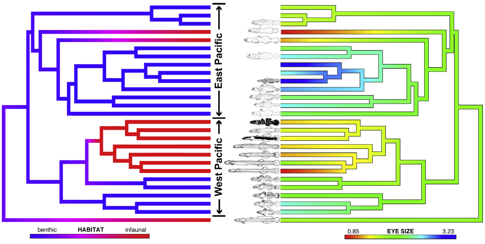
I just learned of this recent article by Ryan Ellingson et al. which makes very neat use of the phytools functions densityMap and contMap for plotting a posterior density from stochastic mapping on a tree, and for mapping a continuous character on the tree (respectively). See Revell (2013) for more details. Below is a reproduction of their figure. On the left is a posterior density from stochastic mapping of 'benthic' vs. 'infaunal' habit; whereas on the right is a projection of the observed or reconstructed values of a continuous character, relative eye size. For more details see the original article, Ellingson et al. (2013).

Click here for larger version.

**Disclaimer: neither densityMap nor contMap can be used (directly) to add tiny line images of fishes to your tree!