New "static" 3D phylomorphospace method

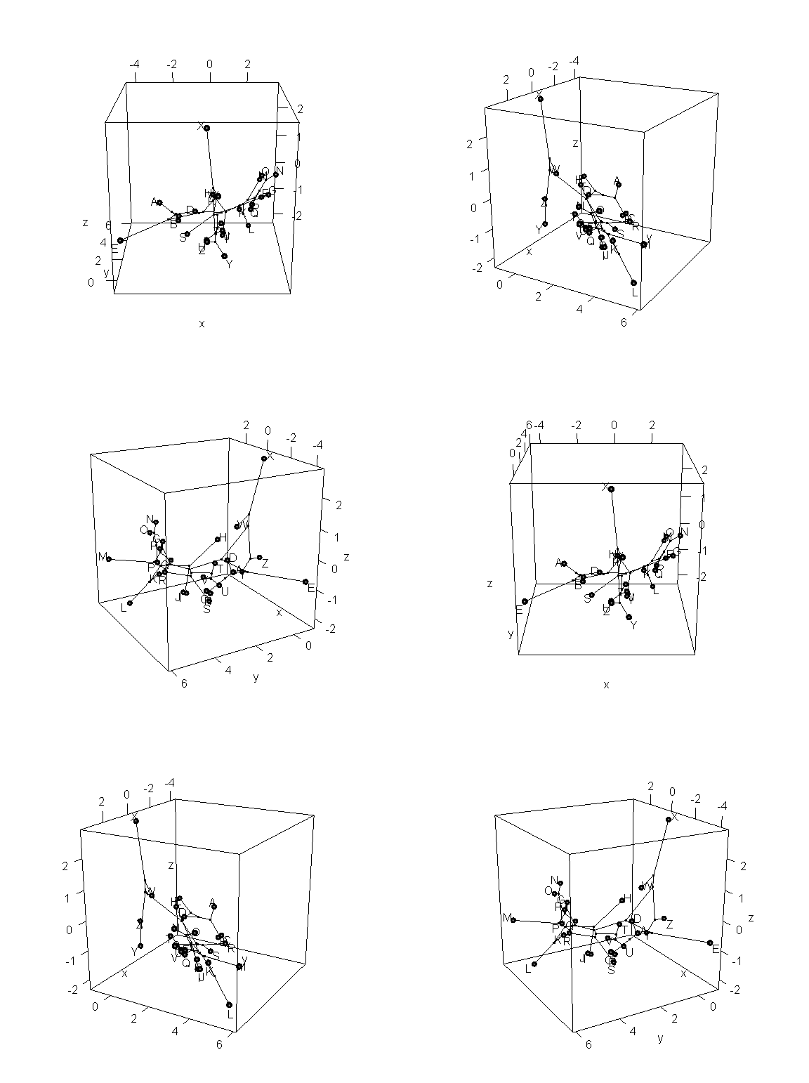
I just developed a new "static" 3D phylomorphospace function; i.e., one that uses R base graphics to simulate three dimensions in a static plot, rather than the rgl library. The advantage of a static plot over a (much more impressive looking) spinning dynamic plot is that it is much easier to modify the plot using base graphics, and it can be exported in standard formats or combined with other plots. Code for this new version is here. The method uses scatterplot3d internally. It is also in a new phytools build (phytools 0.3-40) which can be installed from source.

Here's a quick demo of each method and the different products they create:

> require(phytools)
Loading required package: phytools
> packageVersion("phytools")
[1] ‘0.3.40’
> # simulate tree & data
> tree<-pbtree(n=26)
> tree$tip.label<-LETTERS
> X<-fastBM(tree,nsim=3)
> # first, method="dynamic" (the default)
> xx<-phylomorphospace3d(tree,X)
> movie3d(xx,duration=20,dir=".",movie= "phylomorphospace3d")
Will create: ./phylomorphospace3d.gif
Deleting frames.

> # now, method="static"
> phylomorphospace3d(tree,X,method="static")
> phylomorphospace3d(tree,X,method="static",angle=-30)

Obviously, the dynamic plot makes it a lot easier to see depth in the 3D plot; but the flat plot has the advantage of being something that we can more easily print to a page or combine with other R graphics.

That's it.

plotSimmap(...,type="fan") with node labels

A little while ago, I updated plotSimmap(...,type="phylogram") to (optionally) set the environmental variable "last_plot.phylo" in the environment .PlotEnvPhylo. This has the effect of making plotSimmap fully compatible with nodelabels, tiplabels, edgelabels, and (now) add.scale.bar from the ape package.

The latest version of plotSimmap includes two important updates: (1) now setting the environmental variable "last_plot.phylo", though still optional, defaults to setEnv=TRUE; and (2) setEnv works for both type="phylogram" and type="fan". Since the latter is new - let's try a quick demo showing a stochastic of 'ecomorph' on the tree of Caribbean Anolis ecomorph species, with posterior probabilities from stochastic mapping at internal nodes overlain:

> # load phytools
> require(phytools)
Loading required package: phytools
> packageVersion("phytools")
[1] ‘0.3.38’
> # load anole 'ecomorph' tree
> data(anoletree)
> # this is a stochastic mapped tree - pull tip states
> x<-getStates(anoletree,"tips")
> # conduct stochastic mapping
> trees<-make.simmap(anoletree,x,model="ER",nsim=100, message=FALSE)
> # get the states at ancestral nodes
> aa<-describe.simmap(trees,plot=FALSE)
100 trees with a mapped discrete character with states:
CG, GB, TC, TG, Tr, Tw

trees have 25.79 changes between states on average

changes are of the following types:
...

> # set colors to be used for mapping
> cols<-setNames(palette()[1:6],sort(unique(x)))
> # plotSimmap
> plotSimmap(trees[[1]],cols,type="fan",lwd=3,fsize=0.7)
setEnv=TRUE for this type is experimental. please be patient with bugs
> # add node labels
> nodelabels(pie=aa$ace,piecol=cols,cex=0.4)
> # add legend
> add.simmap.legend(colors=cols,fsize=0.8)
Click where you want to draw the legend

That's ok. Click here for full size.

This update is in a new phytools build (phytools 0.3-38).

New version of plotSimmap (that shouldn't affect anyone - except negatively)

I just posted a new version of the important phytools plotting function plotSimmap. The basic function of plotSimmap is to plot a stochastically mapped tree; however the function is also called internally by a number of other phytools functions such as plotTree, plot.contMap, and plot.densityMap. (This is the basis for the parenthetical part of the post title. More details at the bottom.)

This new version has a number of small updates around the edges - but the biggest update is that it now plots the tree on the original scale, rather than fixing the plotting window at a particular size and then rescaling the tree to the the plotting window. The advantage of this is huge as it makes it much easier to overlay additional plotting elements on our graph.

Now you might ask why would I have fixed the plotting window and rescaled the tree to the plotting window in the first place? Well - good question. The problem is how to figure out what amount of space to leave to the right of the tips of the tree for labels. At the time, the most obvious way to do this was to set the plotting window at a fixed width (say 1.0 unit), and then compute the maximum fraction of that horizontal space to allow for our labels - then rescale the tree to occupy the rest of the space.

Just to quickly demo the consequences of doing it this way:

> library(phytools)
Loading required package: ape
...
> packageVersion("phytools")
[1] ‘0.3.34’
> tree<-pbtree(n=26)
> tree$tip.label<-LETTERS[26:1]
> max(nodeHeights(tree))
[1] 4.31398
> plotTree(tree,mar=c(2,2,2,2))
> axis(1)

First off - by adding the x-axis to the plot we can see that it's not on the original scale, but rescale to a total length of 1.0 (including the tip label). That further predicts that if we had longer tip labels, the length of the plotted tree would also change, and we can see that that is the case:

> tree$tip.label[26]<-paste(c(LETTERS[1],letters[2:12]), collapse="")
> plotTree(tree,mar=c(2,2,2,2))
> axis(1)

So you can see - that in terms of our plotting window, the scale of our tree is actually changing if we get longer tip labels! Oh no. So long as we don't want to add anything to our plotting window this is not a huge issue - and in many situations that will be the case. However as soon as we, say, decide after the fact that we'd like to add a scale bar to our plotted tree, we're in trouble.

Well, I discovered a much better way to handle this problem when I was working on nicer looking labels for the function phenogram. In this method we actually use numerical optimization to find the plotting area that we need to permit our labels & the tree to be plotted. It is based on code modified from the ape package function plot.phylo. Now I've implemented this method in plotSimmap and it is in a new build of phytools (phytools 0.3-36). Let's try it:

> detach("package:phytools",unload=TRUE)
> install.packages("phytools_0.3-36.tar.gz",type="source")
* installing *source* package 'phytools' ...
...
* DONE (phytools)
> library(phytools)
> packageVersion("phytools")
[1] ‘0.3.36’
> tree$tip.label[26]<-LETTERS[1]
> plotTree(tree,mar=c(2,2,2,2))
> axis(1)

> tree$tip.label[26]<-paste(c(LETTERS[1],letters[2:12]), collapse="")
> plotTree(tree,mar=c(2,2,2,2))
> axis(1)

We can see that the scale is the original scale of the tree - and it is retained when we use different sized tip labels.

The new version of plotSimmap also has some other handy updates - for instance, user control of x & y limits. This can be useful in, for instance, adding a legend to the plotted tree. Let's see:

> data(anoletree) # load anole tree
> colors<-setNames(palette()[1:6],sort(unique(getStates(anoletree,"tips"))))
> colors
      CG        GB        TC        TG        Tr        TW
  "black"    "red"  "green3"    "blue"    "cyan" "magenta"
> plotSimmap(anoletree,colors,fsize=0.7,ylim=c(-4, length(anoletree$tip.label)),ftype="i")
> add.simmap.legend(colors=colors,prompt=TRUE, vertical=FALSE)
Click where you want to draw the legend

Pretty cool.

The only problem with this update is that - as mentioned earlier - many of the other plotting functions in phytools rely on plotSimmap internally, and they have been built to accommodate its quirks. Consequently, there is a good chance that this update will break those functions. Fear not - I will work on bringing the rest of phytools into line quickly.

Rooted MRP supertree from rooted triplets

A couple of weeks ago, a phytools user contact me with the following problem:
"My [three taxon] input trees are all rooted. However applying on them the two MRP [Matrix Representation Parsimony supertree] methods available in your package (pratchet and optim.parsimony), the output supertree is always unrooted. Is there anyway to get a rooted tree as output tree? Do you know an MRP method that will allow that (even if it's not implemented in your package)?

Actually, the input trees in mrp.supertree, if rooted, are treated as rooted trees during matrix representation. If this wasn't the case, and input trees were instead automatically unrooted before matrix representation, we would not be able to use triplets as input - because an unrooted triplet contains no information about relationships. However, it is true that the estimated topology is the MP unrooted topology based on the matrix representations of our input trees. This leaves us with the problem of trying to root the final MRP tree, when we don't know the overall outgroup - just the "outgroup" of each triplet.

My solution is that we just attach an artificial outgroup to each of our triplets - making them quartets. Then we perform MRP inference. Then we root the MRP supertree with the artificial outgroup. Then we strip it from our supertree (or set of MP MRP supertrees).

Here's some code to do this:

## first simulate tree for demo
tree<-pbtree(n=26)
tree$edge.length<-NULL
tree$tip.label<-LETTERS[26:1]
## done

## now simulate a set of N triplets
N<-1000 ## big number for the best chance of success
trees<-replicate(N,drop.tip(tree,sample(LETTERS,23)), simplify=FALSE)
class(trees)<-"multiPhylo"
## done

## now, let's attach an outgroup to each triplet
og<-pbtree(n=2)
og$tip.label<-c("NA","outgroup")
og$edge.length<-NULL
trees<-lapply(trees,paste.tree,tr1=og)
class(trees)<-"multiPhylo"
## done

## now our analysis
supertree<-mrp.supertree(trees,method="optim.parsimony", rearrangements="SPR")
if(class(supertree)=="multiPhylo"){
  ## if there is more than one MP tree
  supertree<-lapply(supertree,root,outgroup="outgroup", resolve.root=TRUE)
  supertree<-lapply(supertree,drop.tip,"outgroup")
  supertree<-lapply(supertree,untangle,method="read.tree")
  # this is just for plotting, not the empirical case
  supertree<-lapply(supertree,minRotate,x=setNames(26:1, LETTERS))
  class(supertree)<-"multiPhylo"
  RF<-sapply(supertree,RF.dist,tree2=tree)
} else {
  ## if there is only one MP tree
  supertree<-root(supertree,outgroup="outgroup", resolve.root=TRUE)
  supertree<-drop.tip(supertree,"outgroup")
  supertree<-untangle(supertree,method="read.tree")
  # this is just for plotting, not the empirical case
  supertree<-minRotate(supertree,setNames(26:1,LETTERS))
  RF<-RF.dist(supertree,tree) ## RF distance
}
RF ## RF distances to the true tree
## compare to the true tree
par(mfrow=c(1,2))
plot(tree,no.margin=T)
if(class(supertree)=="multiPhylo"){ plot(supertree[[1]],no.margin=T)
} else plot(supertree,no.margin=T)

How does it do? Well, in this case - not too bad:

> RF ## RF distances to the true tree
[1] 18
> ## compare to the true tree
> par(mfrow=c(1,2))
> plot(tree,no.margin=T)
> plot(supertree,no.margin=T)

(These are almost the same.)

That's it.

Converting a taxonomy to a phylogeny & the problem of branch lengths

A recent R-SIG-phylo subscriber asked:
"I'm trying to build a taxonomic tree from a taxonomic matrix using the function as.phylo.formula of the ape package. It works well but it returns a phylo object without branch length. This is problematic in that it can lead to misleading graphic representation (eg with plot.phylo). For example a dichotomy between two species belonging to the same genus may occur at the same y-coordinate than a dichotomy between two species of different genus."

This turns out to be the case because as.phylo.formula (in the ape package) first uses an algorithm that converts the input taxonomy into a Newick string - specifically without singleton nodes (i.e., nodes with only one descendant) for monogeneric families, monotypic genera, etc. It then reads the Newick string into memory using ape's read.tree to read this Newick string into memory. Having figured this out, addressing this problem in a modified version of as.phylo.formula (code at the end of my email, here - corrected here) was easy. First, I pulled the line of code that prevented the parsing function from creating singleton nodes in the Newick string. Second, I read the tree into memory with the phytools function read.newick, which permits singleton nodes. Third, I assigned unit branch lengths to all edges in this tree with singleton nodes, which guarantees that all internal nodes with the same taxonomic level (e.g., Family) have the same height above the root. Finally, I collapsed all singletons.

Here is a demo of the original function & the modified version:

> library(ape) ## load ape
> data(carnivora)
> t1<-as.phylo.formula(~SuperFamily/Family/Genus/Species, data=carnivora)
> par(lend=2)
> plot(t1,edge.width=2,cex=0.6,no.margin=TRUE)

Right away we can see the problem - nodes at the same taxonomic level are not necessarily at the same height above the root. There's two reasons for this: (1) some taxonomic levels have only one group in the level nested below it (for instance, families with only one genus; genera with only one species, etc.); and (2) compute.brlen, which is used internally by plot.phylo to determine the length of plotted edges with no edge lengths are given, uses the number of descendant leaves to determine the length of edges in the tree - and not all genera (and families, etc.) have the same number of descendant species.

Here is a demo of the modified version that I posted to the listserve:

> source("as.phylo.formula.R")
> t2<-as.phylo.formula(~SuperFamily/Family/Genus/Species, data=carnivora)
> plot(t2,edge.width=2,cex=0.6,no.margin=TRUE)

If we don't like how this looks then in theory we could use a different formula to set our branch lengths, but at least this plot has the property that all nodes at the same taxonomic level have the same height above the root. Cool.

New version of ancThresh with multiple models for the evolution of liability

The phytools package has a couple of different models that implement comparative methods using the threshold model of Wright (1934) and introduced into phylogenetic comparative biology by Felsenstein (2005, 2012). One of these is ancThresh, which fits a multi-state threshold model & uses Bayesian MCMC to estimate ancestral states at internal nodes of the tree. (See here for more information.)

Well, at interesting idea that came up at the NESCent Evolutionary Quantitive Genetics workshop was using other models (such as the OU model) for the evolution of liability on the tree. OU is often used as a model for stabilizing selection. Obviously, in a strict threshold character, liabilities are "hidden" and thus selection should not, in theory, be able to operate directly on liability. Nonetheless, we thought that OU might still be a good model for the evolution of liability under some circumstances. Some example might include, for instance, circumstances where liability has a pleiotropic effect on other non-threshold characters that are under selection; or when liability has natural bounds that create a tendency to revert to an intermediate value (e.g., blood hormone level cannot increase or decrease indefinitely without bounds).

I have just posted a new version of ancThresh that allows the user to fit OU as well as BM. A big question in my mind was how well it would work - given the shortage of data about trait evolution that seems likely to be containing in a two or three state discretely valued trait.

This new version is in a new phytools build (phytools 0.3-33). Let's try it out:

> require(phytools)
Loading required package: phytools
> packageVersion("phytools")
[1] ‘0.3.33’
> require(geiger)
Loading required package: geiger
> ## simulate
> tree<-pbtree(n=100,scale=1)
> l<-fastBM(ouTree(tree,2),a=0.25,sig2=1,internal=TRUE)
> x<-sapply(l,threshState,setNames(c(0,0.5,Inf), LETTERS[1:3]))
> summary(as.factor(x))
A B C
66 100 33
> mcmc<-ancThresh(tree,x[1:100],ngen=200000,control= list(sample=100),model="OU")
**** NOTE: no sequence provided, using alphabetical or numerical order
MCMC starting....
gen 1000
gen 2000
...
gen 200000
> ## first let's see how it does estimating alpha
> burnin<-100000
> ii<-which(mcmc$par[,"gen"]==burnin)
> ps.alpha<-mcmc$par[ii:nrow(mcmc$par),"alpha"]
> mean(ps.alpha)
[1] 1.9842
> pd<-density(ps.alpha,bw=0.4)
> plot(pd,xlab="alpha",main="posterior density of alpha")
> lines(c(2,2),c(0,max(pd$y)),lty="dashed")

> ## now we can see how ancestral states were estimated
> plotTree(tree,setEnv=TRUE,ftype="off")
setEnv=TRUE is experimental. please be patient with bugs
> colors<-setNames(c("blue","green","red"),LETTERS[1:3])
> tiplabels(pie=to.matrix(x[1:100],LETTERS[1:3]),piecol= colors,cex=0.4)
> XX<-t(apply(mcmc$mcmc[ii:nrow(mcmc$mcmc),],2,function(x) summary(factor(x,levels=LETTERS[1:3]))/(nrow(mcmc$mcmc)-ii+1)))
> nodelabels(pie=XX,piecol=colors,cex=0.8)
> nodelabels(pie=to.matrix(x[1:tree$Nnode+100], LETTERS[1:3]),piecol=colors,cex=0.4)

> ## finally, let's see how well liabilities were estimated
> plot(l,colMeans(mcmc$liab[ii:nrow(mcmc$liab),]), xlab="true liability",ylab="estimated liability", main="estimated liability")
> lines(range(l),range(l),lty="dashed")

So, somewhat surprisingly, with as little as three discrete character states we are doing quite well (at least in this instance) of estimated α in the OU model; and we are fairly good at reconstructing ancestral states & liabilities.

That's pretty cool.

New function to strip all the leaves (i.e., tips) off a tree

I today responded to an R-SIG-phylo request for a function that would strip all the leaves (i.e., tips) from a phylogenetic tree - leaving only the internal structure. This can almost be done with drop.tip(...,trim.internal=FALSE); however drop.tip does not allow all tips to be dropped.

I quickly wrote a function that does. Code is here and it is in a new build of phytools (phytools 0.3-22).

Here is a demo of what it does:

> require(phytools)
Loading required package: phytools
> packageVersion("phytools")
[1] ‘0.3.32’
> tree<-pbtree(n=20)
> plotTree(tree,node.numbers=T)

> dt<-drop.leaves(tree)
> plotTree(dt)

NESCent academy "Evolutionary Quantitative Genetics" workshop

I just got back this evening from guest lecturing in a short course at NESCent on "Evolutionary Quantitative Genetics" that Joe Felsenstein and Steve Arnold have been co-teaching for the past few years. Other guest instructors included Trudy MacKay & Pat Phillips (who both came and left before I arrived), as well as Thomas Hansen & Brian O'Meara. Thomas & Brian both led terrifically interesting lectures & discussions. Josef Uyeda, a postdoc on the Harmon lab who is doing some really great comparative methods research, was the course T.A. and lectured as well. (Josef's out-of-date website is here.)

I drew the short straw (kidding) and lectured about the reconstruction of ancestral character states. The figure above is one of my lecture slides showing the likelihood surface for the two nodes above the root as well as the result of a simple hill-climbing optimization. All my lecture slides and details of the four computer labs that I gave are all here, as well as linked off the course materials page. My R tutorials were all created using knitr.

New version of mergeMappedStates; some tutorials in progress

I just posted a new version of the function mergeMappedStates that can "merge" a set of states with only one entry into a new state (basically, change the name of state mapped on the tree). This might be useful for (for example) converting a tree with mapped states a, b, and c into one with two states: a & not-a (coded as 0 & 1, perhaps) for use with densityMap.

This function version is available in a new phytools build (phytools 0.3-21).

Let's try and use the function to do exactly that:

> require(phytools)
Loading required package: phytools
> packageVersion("phytools")
[1] ‘0.3.21’
> ## simulate tree & character data
> tree<-pbtree(n=100,scale=1)
> Q<-matrix(c(-2,1,1,1,-2,1,1,1,-2),3,3)
> colnames(Q)<-rownames(Q)<-letters[1:3]
> x<-sim.history(tree,Q)$states
> ## simulate stochastic histories
> mtrees<-make.simmap(tree,x,nsim=80,model="ER")
make.simmap is sampling character histories conditioned on the transition matrix
Q =
          a        b        c
a -2.433741  1.216870  1.216870
b  1.216870 -2.433741  1.216870
c  1.216870  1.216870 -2.433741
(estimated using likelihood);
and (mean) root node prior probabilities
pi =
        a        b        c
0.3333333 0.3333333 0.3333333
Done.
> ## now let's merge states to make a "a"/"not-a" set of trees
> statea<-mergeMappedStates(mtrees,c("b","c"),"0")
> statea<-mergeMappedStates(statea,"a","1")
> densityMap(statea,type="fan")
sorry - this might take a while; please be patient

I'm also posting a series of tutorials that will form the basis of the computer exercises I will lead this week at the NESCent Academy Evolutionary Quantitative Genetics Workshop in Durham NC this week. I have put draft version of three of these up so far. Check them out here. These tutorials were all created using knitr and have not yet been proofed thoroughly.