New version of plotSimmap (& plotTree) for plotting leftward facing phylogenies

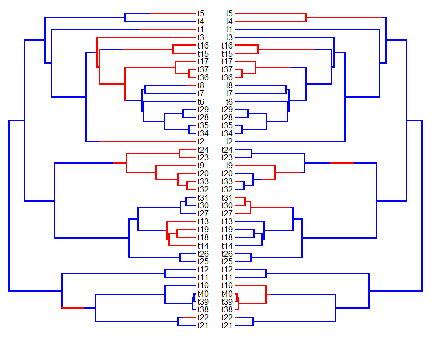
I was working on fixing some bugs in the phytools function phenogram when I suddenly realized how easy it would be to add left-direction plotted trees to the function plotSimmap. We do this with two simple switches. First, when we open a new plotting window we make the x-axis a "reverse axis" by reversing the vector xlim (i.e., such that xlim[1]>xlim[2]). This, without any further changes to the code, will flip all the branches of the tree to run right-to-left. Next, we change the position of the plotted text relative to the end of each leaf in the tree. In a rightward plotted tree, we want this text to be left-aligned and begin where each terminus ends running rightward. A leftward plotted tree needs right-aligned text pointing leftward. This can be changed using the text argument pos, i.e.:

pos<-if(direction=="leftwards") 2 else 4

where 2 and 4 indicate that text should be added to the left of or to the right of the plotting coordinate, respectively.

The updated code for plotSimmap is here. The following is a quick a demo of the new version in action:

> require(phytools)
> source("plotSimmap.R")
> Q<-matrix(c(-1,1,1,-1),2,2)
> tree<-sim.history(pbtree(n=40,scale=1),Q,nsim=2)
> cols<-c("blue","red"); names(cols)<-c(1,2)
> layout(matrix(c(1,2),1,2))
> plotSimmap(tree[[1]],cols,direction="rightwards",lwd=3, pts=F)
> plotSimmap(tree[[2]],cols,direction="leftwards",lwd=3, pts=F)

One known issue is that plotSimmap(...,direction="leftwards",node.numbers=T) doesn't work. This appears to be because the 'graphics' function symbols, which called internally to plot rectangles around each node number, doesn't seem to like a reversed x-axis. If I turn symbols off manually, i.e. just plotting text and no rectangles, the node numbers show up fine.

That's it for now.

New version of phylomorphospace with user control of x & y limits (and other things)

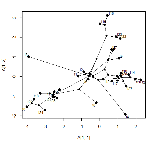
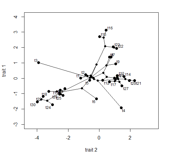
A phytools user today requested user control of x and y limits in phylomorphospace. Currently phylomorphospace sets xlim and ylim based on the range of tip and ancestral values for x & y and this can't be adjusted. It is straightforward to migrate control of this to the user, and I've done this through the "three-dot argument" (i.e., ...). I've also added user control of xlab and ylab, as well as fsize to control the font size of tip labels. fsize is relative to the default font size of textxy(...,cx=0.75).

Code for the new version of phylomorphospace is here, but because the function calls textxy in the 'calibrate' package internally, and phytools imports from calibrate, users will need to either load calibrate to run phylomorphospace from source, or they can install the newest minor build of phytools (phytools 0.2-24).

Here's a quick demo:

> require(phytools)
Loading required package: phytools
...
> packageVersion("phytools")
[1] ‘0.2.24’
> tree<-pbtree(n=30)
> XX<-fastBM(tree,nsim=2)
> par(mar=c(5.1,4.1,2.1,2.1))
> phylomorphospace(tree,XX) # default

> phylomorphospace(tree,XX,ylim=c(-3,4),xlim=c(-4.5,3.5), ylab="trait 1",xlab="trait 2")

That's it.

New version of matchNodes; new minor phytools version

I just made a couple of small updates to matchNodes (1, 2). I wrote this function primarily to be called internally by fastAnc, for which it works just fine, but I've since been frustrated when trying to use it in any task for which it wasn't originally purposed.

More specifically, the function is designed to match nodes between trees that are identical (to some measure of numerical precision) in species, topology, and possibly branch lengths (depending on method). When I tried to use it to match nodes across trees that were identical in core structure, but had different tips added, the function broke down.

The new version should (hopefully) fix this problem. Now, if trees 1 & 2 contains taxa A, B, ..., N, but tree 1 also contains taxa Q, R, S, while tree 2 contains extra taxa T, U, V, the function (using method="distances") should be able to overcome this difference and match corresponding nodes across trees.

Here's a quick demo of what I mean:

> tree<-pbtree(n=10)
> a<-add.random(tree,tips=paste("t",11:15,sep=""))
> b<-add.random(tree,tips=paste("t",16:20,sep=""))
> layout(c(1,2))
> plotTree(a,node.numbers=T)
> plotTree(b,node.numbers=T)

> matchNodes(a,b,"distances")
     tr1 tr2
[1,]  16  16
[2,]  17  NA
[3,]  18  17
[4,]  19  NA
[5,]  20  18
[6,]  21  NA
[7,]  22  19
[8,]  23  20
[9,]  24  21
[10,]  25  NA
[11,]  26  22
[12,]  27  23
[13,]  28  NA
[14,]  29  25
> matchNodes(b,a,"distances")
     tr1 tr2
[1,]  16  16
[2,]  17  18
[3,]  18  20
[4,]  19  22
[5,]  20  23
[6,]  21  24
[7,]  22  26
[8,]  23  27
[9,]  24  NA
[10,]  25  29
[11,]  26  NA
[12,]  27  NA
[13,]  28  NA
[14,]  29  NA

Inspection of these matrices, and the original trees, should show that matchNodes(a,b,"distances") gives the nodes of b (in column 2) that match each node in a; whereas matchNodes(b,a,"distances") gives the reverse.

One little nuance of this method is that we should probably allow it to tolerate inexact matches. This is because adding new edges to the tree, particularly if we then write and read the tree to and from file, will introduce random error to the distances between species and nodes - just because of rounding of branch lengths due to numerical precision of your computer or your file output format specifications. matchNodes has an argument for that: the optional argument, tol. Let's try rounding the branch lengths of each tree, examine the consequences, and then see if it can be fixed by increasing tol:

> a$edge.length<-round(a$edge.length,4)
> b$edge.length<-round(b$edge.length,4)
> matchNodes(a,b,"distances")
     tr1 tr2
[1,]  16  NA
[2,]  17  NA
[3,]  18  NA
[4,]  19  NA
[5,]  20  NA
[6,]  21  NA
[7,]  22  NA
[8,]  23  NA
[9,]  24  NA
[10,]  25  NA
[11,]  26  NA
[12,]  27  NA
[13,]  28  NA
[14,]  29  NA
> # uh-oh!!
> matchNodes(a,b,"distances",tol=0.001)
     tr1 tr2
[1,]  16  16
[2,]  17  NA
[3,]  18  17
[4,]  19  NA
[5,]  20  18
[6,]  21  NA
[7,]  22  19
[8,]  23  20
[9,]  24  21
[10,]  25  NA
[11,]  26  22
[12,]  27  23
[13,]  28  NA
[14,]  29  25

Well, that's pretty cool.

The updated function is here, but it is also in a new minor release of phytools (phytools 0.2-23), along with the new function countSimmap.

Using bind.tip (or bind.tree) on a tree with node labels

Just a quick point of (searchable) clarification for both phytools bind.tip and the ape function bind.tree (bind.tip, after all, uses bind.tree interally; 1, 2). Regardless of whether or not your tree contains node labels (or tip labels, for that matter), the argument where should give the node number (from the matrix tree$edge), at or below which the tip or subtree should be bound.

Node numbers can be seen using:

plotTree(tree,node.numbers=T)
## OR
plot(tree)
nodelabels() # i.e., no arguments

If you want to bind a new tip or subtree to a terminal edge (i.e., an edge ending with a tip), then the 'node number' is just the index of the species in tree$tip.label. We can get this by (for tip name tip) setting where=which(tree$tip.label==tip). Alternatively, if we want to see the node & tip numbers plotted on the tree we could do:

> tree<-pbtree(n=20)
> plot(tree,no.margin=T,label.offset=0.1) # offset may vary
> nodelabels()
> tiplabels()

If adding multiple tips to the tree, remember to keep in mind that each time a new tip is added, the set of node numbers will change. For example:

> tree2<-bind.tip(tree,"t21",where=23,position= 0.5*tree$edge.length[which(tree$edge[,2]==23)])
> ## this just added a new tip halfway along the edge
> ## ending at node 23
> plot(tree2,no.margin=T,label.offset=0.1)
> nodelabels()
> tiplabels()

That's all for now!

Function to count transitions from a mapped tree

To address a user request I just posted a simple function, countSimmap (code here), to count the number of transitions (in total and by type) on a discrete character mapped tree such as a stochastically mapped (i.e., SIMMAP) tree.

Here's a quick demo:

> require(phytools)
> source("utilities.R")
> Q<-matrix(c(-2,1,1,1,-2,1,1,1,-2),3,3)
> colnames(Q)<-rownames(Q)<-c("A","B","C")
> tree<-sim.history(pbtree(n=10,scale=1),Q)
> cols<-setNames(c("blue","red","green"),colnames(Q))
> par(col="white")
> plotTree(tree,ftype="i",lwd=5)
> par(col="black")
> plotSimmap(tree,cols,pts=F,lwd=3,ftype="i",add=T)

> countSimmap(tree,colnames(Q))
$N
[1] 13

$Tr
  A B C
A 0 6 1
B 4 0 2
C 0 0 0

$message
[1] "N is the total number of character changes on the tree"
[2] "Tr gives the number of transitions from row state->column state"

The function is even fast enough to run on quite large trees with lots of transitions, for instance:

> tree<-sim.history(pbtree(n=1000,scale=10),Q)
> system.time(XX<-countSimmap(tree,colnames(Q)))
  user  system elapsed
  0.22    0.00    0.22
> XX
$N
[1] 3762

$Tr
   A   B   C
A   0 623 646
B 605   0 623
C 656 609   0

$message
[1] "N is the total number of character changes on the tree"
[2] "Tr gives the number of transitions from row state->column state"

That's it.

New phytools build and rep() function for "phylo" objects

I just posted a new minor version of 'phytools' (phytools 0.2-22). You can download it here, and install from source.

Relative to the last minor version, this version has only the new function writeAncestors, as well as a function called internally by writeAncestors called repPhylo. repPhylo merely does what the 'base' function rep does for vectors and lists, but for "phylo" objects. This turned out to be annoyingly difficult, until I realized that I could work from this solution on stackoverflow.com.

Here it is, modified for "phylo" objects:

repPhylo<-function(tree,times){
 tree<-
 if(sum(sapply(tree,class)!="list")==0){
   tree
 } else {
     list(tree)
 }
 tree<-rep(tree,length=times)
 class(tree)<-"multiPhylo"
 return(tree)
}

New function to write trees with ancestral states and CIs

A phytools user today requested the ability to output ancestral state estimates (and confidence intervals) to file within a Newick string. Specifically, he had the following suggestion:

It would be great if we could get the ancestral state values as well as the 95CI written in the same tree. So perhaps it is possible to append multiple values to the node like beast does with the 95HPD for divergence time estimates. I looked at the format and it puts multiple values after a node like this [&CI={lower 95%, upper 95%}, ancstate={value}].

Theoretically, this should be straightforward using the optional "phylo" attribute node.label. We could just do, for example:

> tree<-pbtree(n=10)
> x<-fastBM(tree)
> XX<-fastAnc(tree,x,CI=T)
> XX<-lapply(XX,round,2)
> tree$node.label<-paste("[&CI={",XX$CI95[,1],",", XX$CI95[,2],"},ancstate={",XX$ace,"}]",sep="")
> write.tree(tree,digits=2)
[1] "(t1:1.5,(((((t9:0.15,t10:0.15)[&CI={1.061.75}ancstate={1.4}]:0.15,t6:0.3)...

Oops. Unfortunately, this didn't work because write.tree has dropped all of our commas from node.label, even when they're within [...] square parentheses! This is presumably by design to prevent us from using Newick only characters in node labels, although they will be ignored by convention by most applications if given within square brackets.

Luckily, I already have code for tree writing in the form of the phytools function write.simmap, and I thought (rightfully) that it wouldn't be too difficult to modify the code of this function to be able to include ancestral state estimates and CIs in the requested manner.

Well, I ended up building a much more versatile function than I originally intended. writeAncestors (code here) can write trees with ancestors and CIs in "phylip" (i.e., simple Newick) or "nexus" format; it can accept as input the results from ace or fastAnc, and it detects automatically whether or not CIs should be included. In the event that a data vector is provided (that is, tip data instead of the inferred states at nodes) writeAncestors will estimate ancestral states and (optionally) CIs assuming Brownian evolution using fastAnc. In the event that multiple trees, sets of ancestral states, or data vectors are provided, writeAncestors will try to act appropriately.

Here's a quick demo of its simplest usage (some output omitted):

> ls()
[1] "tree" "x"    "XX"  
> source("writeAncestors.R")
> args(writeAncestors)
function (tree, Anc = NULL, file = "", digits = 6,
   format = c("phylip", "nexus"), ...)
NULL
> writeAncestors(tree,XX,digits=2)
(t1:1.47,(((((t9:0.15,t10:0.15)[&CI={1.06,1.75},ancstate={1.4}]:0.15,t6:0.3)...
> # now with a data vector as input
> writeAncestors(tree,x=x,digits=3)
(t1:1.468,(((((t9:0.153,t10:0.153)[&CI={1.057,1.752},ancstate={1.405}]:0.148,t6:0.301)...
> # now to Nexus file (we'll output to screen)
> writeAncestors(tree,x=x,format="nexus")
#NEXUS
[R-package PHYTOOLS, Wed Feb 27 15:47:46 2013]

BEGIN TAXA;
       DIMENSIONS NTAX = 10;
       TAXLABELS
               t1
               t10
               ...
       ;
END;
BEGIN TREES;
       TRANSLATE
               1       t1,
               2       t10,
   ...
       ;
       TREE * UNTITLED = [&R] (1:1.467541,(((((10:0.153423,2:0.153423)[&CI={1.05681,1.75229},ancstate={1.40455}]...
END;

Well, that's it.