Tuesday, August 30, 2011
CRAN Task View: Phylogenetics
Brian O'Meara has very kindly added "phytools" to the CRAN Task View: "Phylogenetics, Especially Comparative Methods" (link here). Thanks to him & thanks to Dave Bapst for suggesting it.
Monday, August 29, 2011
New version of evol.vcv()
Ok, I just posted a new version of evol.vcv() - direct link to code here. The main new feature of this version (v0.2) is that it also computes the variances of the parameter estimates. (The standard errors can then just be computed by taking the square roots.) These variances come from the matrix of partial second derivatives of the likelihood surface at the optimum (i.e., the curvature of the surface), also known as the Hessian matrix. The intuitive relationship between the curvature of the likelihood surface and the uncertainty of our parameter estimates is quite straightforward: if the likelihood surface is very flat (low curvature), then the uncertainty in our parameter estimates is large; conversely if the likelihood surface is very peaked at the optimum (i.e., high curvature), then this implies that uncertainty in our parameter estimates is low.
This function (that is, evol.vcv()) implements the method of Revell & Collar (2009) and was also described in a prior blog post.
In R, normally obtaining the Hessian matrix is easy because the built-in optimizer, optim(), optionally returns its value. Unfortunately, as I outlined in a previous post, this would not do for evol.vcv() because in this function I actually optimized the likelihood with respect to the Cholesky matrices rather than the evolutionary variance-covariances themselves. This was done for computational reasons because the evolutionary variance-covariance matrices (called "rate matrices" in our paper) are subject to annoying constraints which mean that for most random values the likelihood cannot be computed.
The solution, which I figured out yesterday and then implemented today, was to optimize with respect to the Cholesky matrices (as before) - but then differentiate the likelihood surface for the full VCV matrices at the optimum using hessian() in the "numDeriv" package (CRAN page here). This seems to work - and this analysis is implemented in v0.2 of evol.vcv() on my R phylogenetics page. This will also be included in the next version of "phytools".
The variances are not computed by default. To get them, load the present version from source:
> source("http://faculty.umb.edu/liam.revell/phytools/evol.vcv/v0.2/evol.vcv.R") # this should work
> result<-evol.vcv(tree,X,vars=TRUE)
for SIMMAP style tree and data matrix X. Good luck, and please report if this function seems to work properly or not.
Sunday, August 28, 2011
Finding the standard errors from the likelihood surface in evol.vcv()
Today I've been working on returning the variances of the parameter estimates in evol.vcv(). Just to remind the readers of this blog, this function fits two or more instantaneous variance-covariance matrices for the Brownian evolutionary process to different pre-specified parts of a phylogenetic tree. (For more details, see my 2009 paper with Dave Collar or a previous blog post here.)
The first problem that I've run into is that my function performs optimization of the likelihood as a function of the Cholesky decomposite matrices of R. This is because the evolutionary variance-covariance matrix are constrained to be positive semi-definite - a constraint which will cause problems for optim(). My solution to this problem was to optimize the Cholesky decomposite matrix, which does not have this constraint. My issue, then, is that if I return the Hessian matrix of partial second derivatives these will be the curvature of the likelihood surface for the Cholesky matrix elements - rather than for the variances and covariances of our evolutionary rate matrices.
My current plan to solve this involves first using optim() to find the MLEs based on the Cholesky decomposed matrices; and then feeding these parameter estimates along with a likelihood function for the full rate matrices into hessian() in the package "numDeriv". If this works I will soon report the result.
Adding standard errors to evol.vcv()
I haven't done too much programming in the past week or so due (in part) to a disrupted schedule from unusual geological and metereological events of recent days (as well as due to lizards & lots of new activity in my lab); however I am presently adding the calculation of standard errors for parameter estimates to the "phytools" function evol.vcv(). This function is based on Revell & Collar (2009) and was previously described here. In addition to this, on request from Dave Collar, I am planning to next add constraint matrices to test various hypotheses about the evolutionary variance-covariance matrix using this method (for instance, that the evolutionary rates - i.e., variances - are the same in different regimes, but the covariances differ). This will be coming soon.
To all those in Irene's path or wake - stay safe & dry!
To all those in Irene's path or wake - stay safe & dry!
Saturday, August 20, 2011
"phytools" now on CRAN
The "phytools" library is now on CRAN ("phytools" CRAN page here). For most R users, that means it can be installed simply by typing:
> install.packages("phytools")
and then selecting a CRAN mirror.
Note that to install "phytools" this way, Windows users with earlier versions of R will have to upgrade to R 2.13.X; however you can still download the source or a Windows binary from the "phytools" webpage or CRAN page.
> install.packages("phytools")
and then selecting a CRAN mirror.
Note that to install "phytools" this way, Windows users with earlier versions of R will have to upgrade to R 2.13.X; however you can still download the source or a Windows binary from the "phytools" webpage or CRAN page.
Thursday, August 18, 2011
Installing "phytools"
I can see that at least a few visitors to the "phytools" blog have reached this page through the google search "installing phytools" - so I thought I'd say a couple of words about how this can be done at present.
1) Download the package from my R phylogenetics page. If you are a Windows user, you can download the Windows binary (this file ends in ".zip"). If you are a Mac or Linux/Unix user, download the package source (this file ends in ".tar.gz" - actually, you should also be able to install from source in Windows if you are so inclined).
2) Either navigate to the directory containing the "phytools" package installation file, or move the file to your current directory. For the former, you can either use the Windows GUI File->Change dir...; or the R command setwd(). For the latter, the R command getwd() (which returns your current working directory) should be helpful.
3) Now simply enter either:
install.packages("phytools_0.0-7.zip",repos=NULL)
(for Windows installation, assuming the latest version of "phytools"), or:
install.packages("phytools_0.0-7.tar.gz",repos=NULL,type="source")
for installation from source.
4) Finally, to load the "phytools" library, one simply types (as with any other contributed package):
library(phytools)
and you're ready to go!
**Note that I am getting ready to submit "phytools" to CRAN which will have the effect of collapsing steps 1-3 into a single command.**
New phylogenetic ANOVA function with posthoc tests
I just posted a new function to conduct the phylogenetic ANOVA of Garland et al. (1993). Luke Mahler has been doing phylogenetic ANOVA, but wanted to add posthoc comparison of the means between groups. I had previously programmed this in C - but I thought it would be easy enough to do in R as well. Direct link to the code is here. Note that the function, phylANOVA(), borrows a little bit from Luke Harmon's "geiger" function phy.anova(); and the function tTests() (which phylANOVA() calls internally) borrows code from the R "stats" function pairwise.t.test().
The phylogenetic ANOVA is pretty straightforward. First, we fit our ANOVA model (using lm()), and then we compute the F-statistic (using anova()). ANOVA, like most statistical tests, assumes independence - so the P-value returned by anova() will be incorrect. Garland et al.'s simple solution was to obtain the null distribution by simulation, which we can do by first calling X<-fastBM() a single time, and then computing the value of F for each column of X.
The posthoc tests are only a little bit more complicated. Here, we just compute a matrix of t-values for the real data and for each simulated data vector. Note that, for now, the method computes a single pooled standard-deviation which is used for all groups. For each pairwise comparison, we then count the number of simulated t-values with absolute values (for a two-sided test) that are larger than our corresponding empirical t. At the end, though, we have also conducted a large number of tests and that needs to be taken into consideration to control the experiment-wise error rate.
Fortunately in R this is straightforward to accomplish using the p.adjust() function in the "stats" package. p.adjust() implements a whole slew of methods for multiple test correction, and all of them can be called from phylANOVA(...,posthoc=TRUE,p.adj). For instance, standard Bonferroni correction is called by phylANOVA(...,p.adj="bonferroni") and sequential-Bonferroni (the default, also called the Holm-Bonferroni method) is called by phylANOVA(...,p.adj="holm").
Luke reports that the function seems to work properly.
Wednesday, August 17, 2011
New version of phytools (v0.0-7)
I just compiled and posted a new version of the "phytools" package. This can be downloaded from my website, here. In it, I have included the following updates & addition:
1) New function, estDiversity(), described here.
2) Updated versions of read.simmap() & write.simmap() to fix the problem identified by Sam Price by allowing map orders to be read in forward or reverse order (reverse by default - since this is the output of SIMMAP). More on this below.**
3) An updated version of plotSimmap(), described here, that should eliminate the problem of scaling the tree and taxon labels to the plotting window that afflicted earlier versions of this function.
** I also wanted to add a short addendum about reading and writing SIMMAP style trees. By chance, I was contacted today by a user who sent me a SIMMAP style tree (not a stochastic character mapped tree, but a Newick style tree in that format) created (according to them) using BEAST. Anyway, this tree actually turned out to have the forward, not reverse map order! This tree would now have to be read into R using read.simmap(...,rev.order=F) (the default is rev.order=T). To try and relieve some of the confusion around these alternative writing options, I have now created the attribute attr(*,"map.order") which stores the map order of the edges of the input tree (i.e., "left-to-right" or "right-to-left"). This does not affect how the tree is stored in memory, but now is used (unless otherwise specified) by write.simmap() to write the tree with the same format in which it was read.
Tuesday, August 16, 2011
Update to plotSimmap()
In playing around with read.simmap(), I also identified a small issue with the stochastic map plotting function, plotSimmap(). That is, for trees with very short total length (as might be the case with a very slow evolving gene - for instance), the plotted tree is left-aligned in the plotting window and a large amount of white space can be left to right of the tip labels.
To illustrate this, I can first simulate the tree & data:
> require(phytools); require(geiger)
> set.seed(1)
> tree<-rbdtree(b=30,d=0,Tmax=0.1)
> x<-sim.char(tree,model.matrix=list(matrix(c(-10,10,10,-10),2,2)), model="discrete")[,,1]
> mtree<-make.simmap(tree,x)
> cols<-c("blue","red"); names(cols)<-c(1,2)
> plotSimmap(mtree,fsize=0.7,cols)
Which produces the following result:
(border added for illustrative effect).
I had the hardest time trying to resolve this issue; however I finally realized that if I first rescaled the sum of the total tree length and the maximum string width of the longest taxon name (which can be found using strwidth(), once a plotting window has been opened) to 1.0, then the problem is solved.
Let's load the new version of plotSimmap() and try again:
> source("http://faculty.umb.edu/liam.revell/phytools/plotSimmap/v0.6/plotSimmap.R")
> plotSimmap(mtree,fsize=0.7,cols)
Indeed, this looks much better.
Direct link to code for this function is here. I have only tried this on one system - so I would be happy to hear reports that it works on other machines (particularly Mac OS or Linux).
To illustrate this, I can first simulate the tree & data:
> require(phytools); require(geiger)
> set.seed(1)
> tree<-rbdtree(b=30,d=0,Tmax=0.1)
> x<-sim.char(tree,model.matrix=list(matrix(c(-10,10,10,-10),2,2)), model="discrete")[,,1]
> mtree<-make.simmap(tree,x)
> cols<-c("blue","red"); names(cols)<-c(1,2)
> plotSimmap(mtree,fsize=0.7,cols)
Which produces the following result:

(border added for illustrative effect).
I had the hardest time trying to resolve this issue; however I finally realized that if I first rescaled the sum of the total tree length and the maximum string width of the longest taxon name (which can be found using strwidth(), once a plotting window has been opened) to 1.0, then the problem is solved.
Let's load the new version of plotSimmap() and try again:
> source("http://faculty.umb.edu/liam.revell/phytools/plotSimmap/v0.6/plotSimmap.R")
> plotSimmap(mtree,fsize=0.7,cols)

Indeed, this looks much better.
Direct link to code for this function is here. I have only tried this on one system - so I would be happy to hear reports that it works on other machines (particularly Mac OS or Linux).
Discrepancy between read.simmap() and SIMMAP
Sam Price yesterday pointed out to me that my functions read.simmap() and write.simmap() assume the opposite order of the edge states along internal branches created by Jonathan Bollback's program SIMMAP. Yikes! This was news to me, but evidently the mapping ":{1,0.10:0,0.90}" in SIMMAP indicates that the branch started in state 0 and then changed to state 1. Quelle surprise! I had assumed the contrary - that the branch, in this case, started in state 1 (in which it remained for 0.10 units of time) before changing to state 2 for the remainder of the edge.
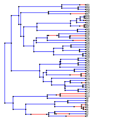
The good news is that misordering the states along the branches is irrelevant for BM based analyses, such as those implemented in brownie.lite() and evol.vcv(). In fact, in the earliest versions of read.simmap(), I discarded this information entirely. However, trees misread in this way look extremely peculiar when plotted using plotSimmap(). For instance, consider the stochastic map below which was created by a colleague using SIMMAPv1.0 and read into R using read.simmap() from the present version of "phytools." Oops!

(In case it's not immediately apparent what is wrong with this image, close examination of almost any branch with a transition shows that this transition occurs at the node, not along the edge as it should.)
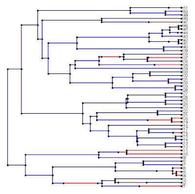
Fortunately, this can easily be solved and I have added it to the latest version of read.simmap(). For backward compatibility, and because I think this ordering makes more sense anyway (no offense intended to JB), I have also retained the option of reading in trees in which the mapped states along an edge are order from root to tip in a left-to-right fashion. This alternative format (still produced by write.simmap() until I fix that too) can be read in by setting the option rev.order=FALSE (default is TRUE).
The fix was very easy to code. Basically, I apply it after reading the tree as before in the following way:
tree$maps<-lapply(tree$maps,function(x) x<-x[length(x):1])
All this does is goes through the list of mapped edges and reverses the ordering of the states, and time spent in each state, for each edge.
This can also be used to convert any tree that has already been read into memory, or even to modify a tree in memory so that it can be written with write.simmap() and then read into another program that accepts standard Newick style SIMMAP format trees.
The new version of read.simmap() is available from my webpage (direct link to code here). I will also put this in the next version of "phytools."
The good news is that misordering the states along the branches is irrelevant for BM based analyses, such as those implemented in brownie.lite() and evol.vcv(). In fact, in the earliest versions of read.simmap(), I discarded this information entirely. However, trees misread in this way look extremely peculiar when plotted using plotSimmap(). For instance, consider the stochastic map below which was created by a colleague using SIMMAPv1.0 and read into R using read.simmap() from the present version of "phytools." Oops!

(In case it's not immediately apparent what is wrong with this image, close examination of almost any branch with a transition shows that this transition occurs at the node, not along the edge as it should.)
Fortunately, this can easily be solved and I have added it to the latest version of read.simmap(). For backward compatibility, and because I think this ordering makes more sense anyway (no offense intended to JB), I have also retained the option of reading in trees in which the mapped states along an edge are order from root to tip in a left-to-right fashion. This alternative format (still produced by write.simmap() until I fix that too) can be read in by setting the option rev.order=FALSE (default is TRUE).
The fix was very easy to code. Basically, I apply it after reading the tree as before in the following way:
tree$maps<-lapply(tree$maps,function(x) x<-x[length(x):1])
All this does is goes through the list of mapped edges and reverses the ordering of the states, and time spent in each state, for each edge.
This can also be used to convert any tree that has already been read into memory, or even to modify a tree in memory so that it can be written with write.simmap() and then read into another program that accepts standard Newick style SIMMAP format trees.
The new version of read.simmap() is available from my webpage (direct link to code here). I will also put this in the next version of "phytools."
Monday, August 15, 2011
New function: estDiversity()
I just posted a "new" function that I actually wrote a while ago for Luke Mahler, and just wanted to return to working on.
Given a tree and a vector, x, containing the biogeographic regions of the tip species, this function computes a vector containing point estimates for the lineage density in each region at each internal node. This is accomplished by first computing the conditional probabilities of being in each region at each internal node (these should probably be the marginal probabilities, but let's just ignore that for a moment). The function then proceeds to take a slice through the tree at the height of that node and compute the marginal probabilities at each "pseudo-node" that is created by the slice bisecting an edge of the tree. The historical lineage density for the node is then estimating by summing these marginal probabilities across the pseudo-nodes and multiplying them by the conditional probabilities at the focal node. This is similar to, but not the same as, the method used in Mahler et al. (2010). Unfortunately, the present implementation requires many calls of the "ape" function ace(), which makes it quite slow. Hopefully, I can improve on this - even if just a little.
Oh yeah - the function is on my R-phylogenetic page (and will also most likely be in the next version of "phytools"). Direct link to the code is here.
Friday, August 12, 2011
Evolutionary rates paper now available online
I just discovered that my paper (with Mahler, Peres-Neto, and Redelings) on the MCMC method for identifying the location of a shift in the evolutionary rate through time is now available online as an "Accepted Article" in Evolution. I have described my work on this method in a number of prior posts (1, 2, 3 ,4, 5, 6, 7, 8, 9, 10). The link to the article is here; however Wiley did not post the supplementary appendix with the article so I will try and post it on my website soon. Check it out!
Thursday, August 11, 2011
New version of "phytools" (v0.0-6)
I just posted a new alpha version of "phytools," version 0.0-6, to my website here.
Here is a list of updates or additions from the previous version:
1. New function map.overlap() that computes the fractional overlap between two stochastically mapped phylogenies (described here).
2. More robust version of brownie.lite() that avoids the problem of "false convergence" in the multi-rate model (described here).
3. New and improved versions of plotSimmap() and plotTree(). These versions have more plotting options including the option to plot without tip labels.
4. Fixed lineage-through-time function ltt(). Bug & fix described here & here, respectively.
Please check it out! Feedback welcome.
Error fixed (I hope!)
I believe I have fixed the error with ltt(), identified here. Basically, the problem seems to have been that, after computing the height above the root of all the nodes and tips in the tree, I was incorrectly counting the number of "events" (that is, increments and decrements of the number of lineages in the tree) which should be the number of nodes + the number of extinct species (that is, assuming that two species never go extinct at exactly the same time, to the extent of numerical precision)+ two (the start and the end). I have now fixed this, which I hope has resolved Rob's problem. Hopefully, the fix has not created other problems, to be discovered.
Note that this function also computes the γ statistic of Pybus & Harvey (2000), but I'm not sure of the validity of this for species with extinct taxa.
Direct link to updated version is here. I will also add this to the next version of "phytools" (which I hope to post on my website today or tomorrow).
Error with ltt()
Rob Lanfear has identified a problem with the function ltt() in "phytools" when the tree includes extinct lineages. For instance, take the following tree with 20 extant taxa:

With the present version of ltt(), we get:

which is obviously incorrect. We can substituted v0.3 of the function and try again:
> source("http://faculty.umb.edu/liam.revell/phytools/ltt/v0.3/ltt.R")
> ltt(tree,log.lineages=F)

and this seems to solve the problem. I will try and fix the most recent version (which corrected some bugs from v0.3 as well as adding additional functionality) and this will be included in the next version of "phytools." Thanks to Rob for finding this problem.
Note that the tree above was simulated using Tanja Stadler's neat package "TreeSim."
Subscribe to:
Posts (Atom)