New method for "co-phylogenetic" plotting

I just added a function to plot co-phylogenetic trees (that is, trees which have been plotted to maximize the vertical alignment of tips). This is not meant to displace or replace the function cophyloplot from the ape package, just as an alternative. It also does not (yet) contain the full range of plotting options that can be accesses using (for example) plot.phylo or plotSimmap (neither of which are used internally by this function. Consequently, though the function produces a nice visualization (in my opinion) - it is not particularly flexible.

It works in the following way. First, the function cophylo takes two trees and an “association” table to (by default) try to rotate all the nodes of the tree so that the match the specified association as closely as possible. It returns an object of class "cophylo" which is then plotted using an S3 plotting method that I have written for that object class.

Here is a demo using a simulated tree & association matrix:

library(phytools)
source("http://www.phytools.org/cophylo/v0.1/cophylo.R")
N<-20
tips.tr1<-replicate(N,paste(sample(LETTERS,1),"._",
    paste(sample(letters,round(runif(n=1,min=4,max=8))),
    collapse=""),sep=""))
tips.tr2<-replicate(N,paste(sample(LETTERS,1),"._",
    paste(sample(letters,round(runif(n=1,min=4,max=8))),
    collapse=""),sep=""))
tr1<-pbtree(n=N,tip.label=tips.tr1)
tr2<-pbtree(n=N,tip.label=sample(tips.tr2))
assoc<-cbind(tips.tr1,tips.tr2)
## here is our association matrix
assoc

##       tips.tr1      tips.tr2     
##  [1,] "W._dlwm"     "A._fzgam"   
##  [2,] "X._escrndyh" "W._szwf"    
##  [3,] "E._bqnfgamo" "S._yxau"    
##  [4,] "U._flhus"    "X._awegv"   
##  [5,] "A._wtidb"    "P._xeiuglq" 
##  [6,] "E._fgcjur"   "P._fpoqim"  
##  [7,] "D._dvsnroq"  "C._otvsn"   
##  [8,] "B._ampg"     "P._mxbra"   
##  [9,] "S._jtugw"    "Y._nqum"    
## [10,] "F._lkein"    "K._qvrml"   
## [11,] "D._wsahm"    "J._ecslngd" 
## [12,] "K._tjwybe"   "R._vxedtwu" 
## [13,] "W._kesxcfy"  "J._vycwi"   
## [14,] "J._dluaog"   "S._pebgjt"  
## [15,] "O._widztm"   "N._gjeklr"  
## [16,] "R._iabcfg"   "O._yhmpdwle"
## [17,] "U._vykna"    "V._evuls"   
## [18,] "L._krumtvwa" "J._tzocbar" 
## [19,] "R._gitlsuy"  "B._imgyxv"  
## [20,] "K._yajemc"   "X._vctdwuf"

Now let's run our functions. First without rotation, then with rotation (the default):

## no rotation
obj<-cophylo(tr1,tr2,rotate=FALSE,assoc=assoc)
obj

## Object of class "cophylo" containing:
## 
## (1) 2 (possibly rotated) phylogenetic trees in an object of class "multiPhylo".
## 
## (2) A table of associations between the tips of both trees.

plot(obj)

## with rotation
obj<-cophylo(tr1,tr2,assoc=assoc)
obj

## Object of class "cophylo" containing:
## 
## (1) 2 (possibly rotated) phylogenetic trees in an object of class "multiPhylo".
## 
## (2) A table of associations between the tips of both trees.

plot(obj)

If we don't specify an association matrix, then the function assumes that the tip labels are meant to match exactly. We also do not need to use trees that are ultrametric. Here is an example that demonstrates both points:

tr1<-rtree(n=30)
tr2<-rtree(n=30)
obj<-cophylo(tr1,tr2)
plot(obj)

That's it!

Ilhabela macroevolution final t-shirt design (& other stuff)

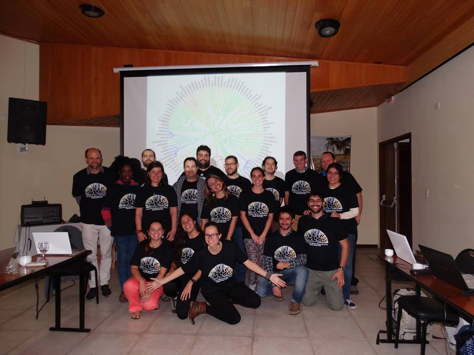
Since our second Latin American Macroevolution workshop - this year held in Ilhabela, Brazil - is now done, I thought I'd post a quick update on our final t-shirt design. I posted a prototypical version earlier on this blog; however subsequent to making that design we decided to switch from a continuous character map, so a stochastically mapped discrete character using a Brazilian flag color palette. Here is the result:

library(phytools)
## read in tree
tree<-read.tree(text="(((t2:0.41,((t15:0.116,(t68:0.03,t69:0.03):0.086):0.18,(((t43:0.058,((t97:0.001,t98:0.001):0.03,t67:0.032):0.027):0.072,((t95:0.002,t96:0.002):0.028,t70:0.03):0.1):0.072,t5:0.202):0.094):0.114):0.004,((((((t76:0.022,t77:0.022):0.05,(t61:0.034,t62:0.034):0.038):0.03,((t91:0.005,t92:0.005):0.021,t75:0.026):0.076):0.083,t9:0.185):0.2,(((t10:0.16,((t30:0.078,(t80:0.014,t81:0.014):0.064):0.005,((((t99:0,t100:0):0.03,(t73:0.027,t74:0.027):0.004):0.004,t60:0.034):0.011,t51:0.045):0.038):0.077):0.054,(t7:0.188,(((t54:0.039,(t84:0.01,t85:0.01):0.028):0.09,t14:0.129):0.027,(t31:0.076,(t57:0.034,t58:0.034):0.042):0.08):0.032):0.026):0.083,(((t93:0.004,t94:0.004):0.002,t90:0.006):0.204,((t71:0.029,t72:0.029):0.101,t13:0.13):0.08):0.086):0.088):0.024,((t3:0.26,(t4:0.207,((t32:0.074,(t49:0.049,t50:0.049):0.026):0.099,(((((t78:0.018,t79:0.018):0.025,t52:0.042):0.054,t21:0.096):0.034,t12:0.13):0.01,(t33:0.074,((t65:0.032,t66:0.032):0.009,t53:0.041):0.032):0.067):0.032):0.034):0.053):0.016,(t11:0.154,(t26:0.086,((t55:0.036,t56:0.036):0.018,t46:0.054):0.032):0.068):0.122):0.132):0.004):0.086,((((t8:0.186,((t16:0.114,(t24:0.088,t25:0.088):0.027):0.008,(t40:0.068,t41:0.068):0.054):0.063):0.08,(((((t47:0.051,t48:0.051):0.044,t22:0.095):0.009,t18:0.104):0.053,((t19:0.102,((t83:0.012,(t86:0.01,t87:0.01):0.002):0.054,t42:0.068):0.034):0.018,((t23:0.09,(t28:0.085,t29:0.085):0.005):0.011,(t38:0.068,t39:0.068):0.034):0.018):0.038):0.03,((t44:0.057,t45:0.057):0.048,t17:0.104):0.082):0.08):0.082,(((t59:0.034,(t82:0.014,(t88:0.009,t89:0.009):0.004):0.021):0.13,(((t34:0.073,t35:0.073):0.013,t27:0.086):0.015,(t63:0.033,t64:0.033):0.068):0.064):0.059,(t6:0.19,((t36:0.072,t37:0.072):0.028,t20:0.1):0.09):0.033):0.125):0.098,t1:0.446):0.054);")
## create transition matrix
Q<-matrix(c(-3,1,1,1,
    1,-3,1,1,
    1,1,-3,1,
    1,1,1,-3),4,4)
rownames(Q)<-colnames(Q)<-letters[1:4]
## simulate stochastic character history
tree<-sim.history(tree,Q)

## Done simulation(s).

cols<-setNames(c("#309030","#182B78","#F0F0F0","#F0C000","#134913"),
    letters[1:4])

Now we're ready to make our plot:

layout(mat=matrix(c(1,2),2,1),heights=c(0.8,0.2))
par(bg="black")
par(fg="white")
plotSimmap(paintSubTree(tree,Ntip(tree)+1,"1"),type="fan",
    ftype="off",colors=setNames("white","1"),lwd=6,part=0.5)

## setEnv=TRUE for this type is experimental. please be patient with bugs

plotSimmap(tree,colors=cols,type="fan",ftype="off",lwd=4,
    add=TRUE,part=0.5)

## setEnv=TRUE for this type is experimental. please be patient with bugs

plot.new()
text(0.5,0.5,"Latin American Macroevolution Workshop\nIlhabela Brazil 2015",
    col="white",cex=2.1,font=2)

Once again, if we want to produce a high quality version without the aliasing that we see in the plot above, we can do that easily by exporting as a pdf:

pdf(file="brazil-colors.pdf",width=8,height=4.75)
layout(mat=matrix(c(1,2),2,1),heights=c(0.8,0.2))
par(bg="black")
par(fg="white")
plotSimmap(paintSubTree(tree,Ntip(tree)+1,"1"),type="fan",
    ftype="off",colors=setNames("white","1"),lwd=6,part=0.5)

## setEnv=TRUE for this type is experimental. please be patient with bugs

plotSimmap(tree,colors=cols,type="fan",ftype="off",lwd=4,
    add=TRUE,part=0.5)

## setEnv=TRUE for this type is experimental. please be patient with bugs

plot.new()
text(0.5,0.5,"Latin American Macroevolution Workshop\nIlhabela Brazil 2015",
    col="white",cex=2.1,font=2)
dev.off()

## png 
##   2

This PDF can be found here.

Note that since the plot above used a stochastic simulation, the realized t-shirt design was actually slightly different (see below).

Finally, the course was a huge success (in my opinion). Certainly, the students we had this year (like last year) were fantastic, and they even seemed to like the t-shirts:

(Click for a larger version.)

Thanks to the TAs, my co-instructors Luke Harmon & Mike Alfaro, and, of course, the excellent students. We're already looking forward to next year!

New version of phytools (phytools 0.4-60) on CRAN

Yesterday I submitted a new version of phytools to CRAN (phytools_0.4-60), and this afternoon it was accepted & posted.

There are no major new methods to report in this version over the last CRAN release of phytools; however I have made a number of different updates to a variety of frequently (& infrequently) used functions. Among these:

1. An update to plot.contMap to permit user control of the legend text.

2. A bug fix in phenogram for when ftype="off" (i.e., the traitgram is being plotted without labels.

3. A bug fix for ltt for an input tree with node labels.

4. A long overdue update to the ancestral state reconstruction function rerootingMethod to permit trees with multifurcations.

5. New S3 print & plot methods, and a new custom object class, for the phytools lineage-through-time function ltt (here).

6. A minor bug fix in the phytools function writeAncestors.

Finally, 7. an update to ltt to permit the lineage-through-time plot to include an overlain phylogeny (1, 2).

This new package update was also necessited by changing CRAN policies which now require that all internally used functions from core R packages, such as graphics, utils, and methods also be imported into the namespace and specified in the DESCRIPTION file - so you can also see that on the phytools CRAN page.

That's all for now! Hopefully there will be more interesting updates to report for the next new CRAN version of phytools.

New feature in LTT plotter to overlay plotted tree

I just posted a version of the function ltt (Lineage-Through-Time) that permits the user to automatically overlay the phylogeny on a lineage through time plot. I wrote about how to do this manually in a previous post. This update is part of a new version of phytools, phytools 0.4-60, which has been submitted to CRAN - but for now can also be downloaded and installed from source from the phytools page.

Here is a demo of how it works:

library(phytools)
packageVersion("phytools")

## [1] '0.4.60'

tree<-pbtree(n=26,tip.label=LETTERS)
## simulated tree:
plotTree(tree)

obj<-ltt(tree,plot=FALSE)
## object of class "ltt"
obj

## Object of class "ltt" containing:
## 
## (1) A phylogenetic tree with 26 tips and 25 internal nodes.
## 
## (2) Vectors containing the number of lineages (ltt) and branching times (times) on the tree.
## 
## (3) A value for Pybus & Harvey's "gamma" statistic of -1.0815, p-value = 0.2795.

## regular ltt plot
plot(obj)

## overlay tree on plot
plot(obj,show.tree=TRUE)

That's all there is to it. At present I don't have it set up to change the color of the tree - however, there is an option to increase or decrease the transparency:

plot(obj,show.tree=TRUE,transparency=0.2)

That's it for now. Stay tuned for another post detailing the updates in the latest phytools version.