New version of tree simulator with taxa & time stops (and both)

This is not what I set out to do when I reopened the function pbtree that I use often, but have barely looked at in two years (that'll come in a future post); however last night & this morning I thought it would be neat to add a time-stop criterion to the existing taxa-stop in the stochastic pure-birth tree simulator in phytools, pbtree. Having done that, I realized it would be straightforward to just use rejection sampling to simulate simultaneously conditioning on both N & t.

Tree simulation is much less complicated than it might seem at first glance. The waiting time between speciation events on a Yule tree are exponentially distributed with the rate parameter, λ = b × m where m is the number of "open" edges. Having drawn a random waiting time, we first add the wait time to all the open edges of the tree; and then we speciate any of the open edges at random. We repeat this procedure until we reach a set number of tips or time.

One way to condition on both the total time & the number of tips is to repeatedly simulate trees under the time-stop criterion until a tree with the correct number of tips is obtained. In theory this could take a long time, even if we use a birth-rate where E[N]=e^b×t. This is because the variance on stochastic pure-birth trees is very large. For instance:

> source("pbtree.R")
> # simulate 1000 trees with a time-stop
> trees<-pbtree(b=1,t=log(100)-log(2),nsim=1000)

(I use t=log(100)-log(2) because this is the amount of time we expect will result in 100 tips given b=1, on average.)

> # how many tips in each tree?
> N<-sapply(trees,function(x) length(x$tip.label))
> mean(N)
[1] 100.499
> var(N)
[1] 4946.41
> hist(N,0:17*25,col="grey",xlab="frequency",ylab="number of tips",main=NULL)

Nonetheless, pbtree is sufficiently speedy that it is still possible to simulate using both a taxon & time-stop. Here's a demo:

> system.time(tree<-pbtree(b=1,t=log(100)-log(2),n=100))
simulating with both taxa-stop (n) and time-stop is
performed via rejection sampling & may be slow

  126 trees rejected before finding a tree

   user  system elapsed
   0.61    0.00    0.61
> tree

Phylogenetic tree with 100 tips and 99 internal nodes.

Tip labels:
        t17, t18, t69, t70, t21, t12, ...

Rooted; includes branch lengths.

Cool.

The code for the new version of pbtree is here.

Some performance tests of make.simmap

The phytools function make.simmap performs stochastic mapping following Bollback (2006); however it does not implement a full hierarchical Bayesian model because stochastic maps are drawn conditional on the most probable value of the transition matrix, Q, found using maximum likelihood (given our data & tree - which are also assumed to be fixed). This is different from what (I understand) is implemented for morphological characters in the program SIMMAP, in which stochastic character histories & transition rates are jointly sampled, with a prior distribution on the parameters of the evolutionary model specified a priori by the user. Conditioning on the MLE(Q) (rather than integrating over the posterior distribution of Q) would seem to make what is done in make.simmap an empirical Bayes (EB) method.

From stochastic mapping we can compute posterior probability distributions on the number transitions between each pair of states; the total number of transitions; and the proportion of or total time spent in each state on the tree. (We can also get posterior probabilities of each state at internal nodes - i.e., ASRs - but these are boring & make.simmap does fine with this, so I won't focus on that here.)

I anticipated that make.simmap would have the following properties:

1. The point estimates of our variables of interest should be fine - i.e., unbiased and as good as the full hierarchical model.

2. The variance around those estimates computed from the posterior sample of stochastically mapped trees should be too small. This is because we have effectively ignored uncertainty in Q by fixing the transition matrix at its most likely value.

Finally, 3. the discrepancy in 2. should decline asymptotically for increasing tree size. This is because the more tips we have in our tree, the more information they will contain about the substitution process. In other words, the influence of ignoring uncertainty in Q should decrease as the information in our data about Q is increased.

These predictions are intuitive, but at least 1. & 2. are also typical of EB generally. Number 3. just seems sensible.

Unfortunately, since stochatic mapping is a computationally intensive Monte Carlo methods, testing these predictions is somewhat time consuming - and what I'll show now is only a very limited test. Basically, I simulated trees & data containing either 100 or 200 tips (and then 40 tips, see below) using pbtree and sim.history. The data are a binary character with states a and b, and the substitution model is symmetric - i.e., Q_a,b = Q_b,a. I wanted to see if our variables were estimated without (much) bias; and if (1-α)% CIs based on the posterior sample included the observed values (which we know from simulation, of course) the correct fraction of the time (e.g., 95% of the time for α = 0.05).

OK - I won't give all the code for simulation, but here is a figure showing a visualization of a single example result from one simulated 100-taxon tree & dataset. The panels give the transition rates between state, the total changes, or the relatively time spent in state a. (Since this last quantity is expressed as a proportion of the total time, the time spent in b is just 1 minus this.) The vertical dashed line is the value of each variable on the true tree.

This result was chosen at random, believe it or not (actually, it was the last of 100 simulations under the same conditions), but it happens to be a replicate in which make.simmap did really quite well.

Here is a table containing a summary of the first 10 of 100 simulations using 100-taxon trees, just to give the reader a sense of the data being collected. Hopefully the column headers are obvious.

> result[1:10,1:4]
   a,b low.a,b mean.a,b high.a,b
1    8       2    5.820       11
2    7       3    5.750       10
3    9      10   19.155       30
4   15      11   15.660       20
5    5       5    8.780       12
6    4       2    7.030       14
7   13       9   11.940       16
8    8      11   17.420       25
9    5       3    6.810       12
10   7      10   18.650       28
> result[1:10,5:8]
   b,a low.b,a mean.b,a high.b,a
1   16      12   15.070       19
2   10       7   10.410       14
3   21      16   25.510       34
4    5       2    5.940       12
5    5       3    5.875       10
6   17      13   17.265       22
7    8       5    8.295       12
8   18      10   17.490       24
9   12       7   11.005       15
10  18       9   18.150       26
> result[1:10,9:12]
    N low.N mean.N high.N
1  24    15 20.890     28
2  17    11 16.160     22
3  30    32 44.665     60
4  20    15 21.600     29
5  10    11 14.655     20
6  21    16 24.295     32
7  21    14 20.235     27
8  26    25 34.910     45
9  17    13 17.815     25
10 25    27 36.800     48
> result[1:10,13:16]
   time.a low.time.a mean.time.a high.time.a
1   0.229      0.196       0.244       0.310
2   0.296      0.225       0.289       0.361
3   0.335      0.271       0.392       0.541
4   0.762      0.651       0.743       0.805
5   0.364      0.305       0.394       0.467
6   0.182      0.173       0.230       0.322
7   0.485      0.410       0.456       0.505
8   0.320      0.333       0.441       0.549
9   0.201      0.209       0.284       0.397
10  0.260      0.294       0.423       0.565

We can first check to see if the point estimates, obtained by averaging over stochastic maps for each simulation, give good estimates of the generating values for the variables that we are interested in. So, let's take the transitions from b to a as an example:

> plot(RR[,"b,a"],RR[,"mean.b,a"],xlab="true b->a", ylab="mean(b->a)")
> lines(c(0,max(RR[,"b,a"],RR[,"mean.b,a"])), c(0,max(RR[,"b,a"],RR[,"mean.b,a"])),lty="dashed")

We see that our point estimates track the known true number of transitions fairly well - so clearly we're not doing too bad with regard to bias. Let's quantify it across all the variables of interest:

> mean(RR[,"mean.a,b"]-RR[,"a,b"])
[1] 1.97765
> mean(RR[,"mean.b,a"]-RR[,"b,a"])
[1] 1.5159
> mean(RR[,"mean.N"]-RR[,"N"])
[1] 3.49355
> mean(RR[,"mean.time.a"]-RR[,"time.a"])
[1] 0.005261939

There looks to be a slight upward bias in the estimated number of substitutions - but this might just be due to the fact that our posterior sample is truncated at 0. (I.e., we might do better with the mode or median from the posterior sample instead of the arithmetic mean.) The time spent in a (and thus also b) seems to be estimated unbiasedly.

We can also ask, for instance, if the interval defined by [α/2, 1-α/2]% of the posterior sample includes the generating values (i.e., from our simulated tree) (1-α)% of the time. Setting α to 0.05:

> colMeans(on95)
   a,b    b,a      N time.a
  0.76   0.89   0.79   0.82

we see that indeed, and as expected, the variance on our variables is too small. Not way too small - what should be our 95% CI is actually our "76-89% CI" for these trees & data - but too small nonetheless.

Finally, prediction 3. Since I expect that the fact that our CIs are too small is due to fixing Q rather than integrating over uncertainty in Q (as we'd do in the full hierarchical model), I predicted that the variance of our parameters should asymptotically approach the true variance for more & more data. To "test" this, I simulated trees with 200 taxa and repeated the analyses above.

Here is one representative result, as before:

And let's check the average outcome across 100 simulations:

> colMeans(on95)
   a,b    b,a      N time.a
  0.85   0.87   0.77   0.86

To be honest, I was kind of surprised not to have found a larger effect here, so I decided to go in the other direction - and try simulating with quite small trees, say 40-taxa. First, here's a representative set of visualizations of the posterior densities/distributions for our focal variables in one randomly chosen simulation:

And here is our measure of the fraction of results on the (ostensible) 95% CI from the posterior:

> colMeans(on95)
   a,b    b,a      N time.a
  0.83   0.75   0.73   0.74

This result does seem to support premise 3., although, as for when we went from 100 to 200 tips, the effect of going from 100 to 40 is not especially large.

I should also be careful to note that this doesn't mean, of course, that we don't get much better parameter estimation from larger trees with more data - we do. It is just to say that convergence of our [α/2, 1-α/2]% to the true (1-α)% is flatter than I expected as sample size is increased, if it happens at all.

So, in summary - make.simmap does pretty well in point estimation. 95% CIs from the posterior sample will be too small - but not way too small, even for relatively small trees.

What's the way forward from here? Well, it would be nice to compare to SIMMAP, as I'm not aware of this kind of analysis having been done & published for morphological traits. In addition, there are steps that could be taken with make.simmap other than going to the full hierarchical model - for instance, instead of fixing Q at its MLE, I could use MLE(Q) to parameterize a prior probability distribution of the transition matrix. This would still be EB, just of a different flavor.

OK - that's all for now!

Small bug fix in make.simmap for multiple input trees

For some reason in a recent version of make.simmap with multiple input trees I had the brilliant idea that it would be smart to print Done. at the end of every set of simulations. The consequence of that self-inflicted wound is a fatal error when multiple input trees are read in! This is because I evaluate the optional argument message inside a conditional if(class(tree)=="phylo"), but then try to compute if(message) message("Done.") outside that if statement. The result is that, after calling itself recursively many times, at the very end make.simmap fails when trying to evaluate if(message). Oh no!

I also identified a different, non-fatal bug that affected make.simmap(...,nsim=1) for multiple input trees. This bug came about because for every input tree I called make.simmap(...,nsim) and then non-recursively unlisted the resulting object. The problem is that if nsim=1 then the non-recursive unlisting unlists the tree object. Oops!

Both of these bugs are in the latest CRAN release, which is annoying - but I have posted fixed code for make.simmap here and an updated build of phytools (phytools 0.2-42).

Estimating ancestral states when species values are uncertain or unknown, part II

Last month I described a method whereby stochastic mapping can be used to estimate ancestral states when tip states are uncertain or unknown. An ancillary benefit of this approach (now implemented in the 'phytools' function make.simmap) is that it can also be used to get posterior probabilities on the states for those uncertain or unknown terminal taxa.

Well, the same general tactic can be used to get marginal ancestral state reconstructions using likelihood. (I.e., the empirical Bayes marginal reconstructions of Yang 2006. Yang calls these "empirical Bayes" reconstructions, because they are Bayesian posterior probabilities - but they treat the empirical tree & MLE model of evolution as if they are known without error.)

Marginal ancestral state reconstruction using the re-rooting method of Yang is implemented in the phytools function rerootingMethod. This method works by taking advantage of the fact that the normalized likelihoods at the root node from the pruning algorithm are the same as the (posterior) probabilities of each state at that node (Yang 2006) - that is, assuming our model of evolution is symmetric. That means that we should be able to re-root the tree at each internal node and compute the marginal ancestral states (posterior probabilities) for that node via one post-order tree traversal.

When tip nodes are unknown or uncertain this is treated as a prior probability distribution on the state for the tip. For example, we might specify a totally unknown tip as having an equal prior probability of being in any of the states; or we might know that a tip is in state a or b, but not c, in which case we might specify a flat prior probability distribution but only on a & b, with state c getting a prior probability of 0. We can then use these prior probabilities just as we would the conditional likelihoods of internal nodes during the pruning algorithm.

To get the posterior probability of tip nodes is simple - we just re-root the tree at the tip of interest and then compute the normalized conditional likelihoods for that node. These are are empirical Bayes posterior probabilities for the tip states, given our data & fitted model of evolution.

The code for this new function is here; however if you want to try it out, you might want to get the new non-CRAN build of phytools (phytools 0.2-41) because this function calls some internal functions of the phytools package (which it won't be able to do if you just load the function from source).

Here's a quick demo of how it works:

> require(phytools)
Loading required package: phytools
> # simulate a tree & data
> tree<-pbtree(n=20,scale=1)
> Q<-matrix(c(-1,1,1,-1),2,2)
> rownames(Q)<-colnames(Q)<-letters[1:2]
> x<-sim.history(tree,Q)$states
> plot(tree,no.margin=T,edge.width=2,label.offset=0.02)
> tiplabels(pie=to.matrix(x,letters[1:2])[tree$tip.label,], piecol=c("blue","red"),cex=0.6)
> # ok, get the marginal ASRs without uncertainty
> PP<-rerootingMethod(tree,x)
> nodelabels(pie=PP$marginal.anc,piecol=c("blue","red"), cex=0.6)

OK, now let's pretend that some of our tip states are uncertain/unknown:

> # now let's pretend we have some uncertainty in
> # our tip states
> Pr<-to.matrix(x,letters[1:2])
> Pr["t3",]<-c(0.5,0.5)
> Pr["t12",]<-c(0.5,0.5)
> Pr["t19",]<-c(0.5,0.5)
> QQ<-rerootingMethod(tree,Pr)
> tiplabels(pie=QQ$marginal.anc[tree$tip.label,], piecol=c("blue","red"),cex=0.6)
> nodelabels(pie=QQ$marginal[as.character(1:tree$Nnode +length(tree$tip)),],piecol=c("blue","red"),cex=0.6)

The posterior probabilities for the tip nodes here also seem totally sensible. For example, tip t3 is on the end of a very long branch - so the posterior probability is dominated by the prior. By contrast, tip t19 is on a short branch & nested within a clade in state b (i.e., red); and thus the empirical Bayes posterior probability that t19 is also in state b is very high - as shown in the figure.

Pretty cool!

phytools 0.2-40 on CRAN

A new version of phytools is now available on CRAN. I submitted the last CRAN version of phytools March 20th, so there are not a huge number of updates in the present version - but some of them are important or very cool, so I decided to get the new phytools version on CRAN anyway. Over the new few days, Windows & Mac OS X binaries should be built and then gradually percolate through the CRAN mirror repositories.

Here are some of the updates in this version relative to phytools 0.2-30, the last CRAN phytools version:

1. A new function to get the marginal ancestral state reconstructions of a discrete character using the re-rooting method.

2. A new function to summarize the results of stochastic mapping (1, 2, 3).

3. An update to make.simmap to allow uncertain tip states.

4. A small update to phylosig in the calculation of P-values.

5. An update to make.simmap to allow it to performing mapping on a set of input trees, for instance from the posterior distribution of a Bayesian analysis.

6. An important bug fix in make.simmap for asymmetric substitution models (e.g., model="ARD").

7. Finally, a new, totally rewritten version of phylomorphospace that also allows users to show a mapped discrete character on the tree.

Please report any bugs or issues.

New completely re-written version of phylomorphospace with mapped discrete trait

I just posted a new, completely re-written version of phylmorphospace - the phytools function that does a projection of the tree into a two dimensional morphospace. Since I wrote the original version way back in 2010, and the guts of the function had persisted largely unchanged since that time, this was probably overdue.

There was no major issue with the prior version; however I wanted to add some features and realized that the code could be a lot nicer - so I decided to re-write the function (pretty much) from scratch.

Phylomorphospace plots are pretty easy in principle. We just need to supply tip states & compute or supply all the states at internal nodes. Having done that, we can just plot all the tip & node states in our bivariate morphospace, and then add edges connecting all parent & daughter nodes.

Source code for the updated version of phylomorphospace is here; I have also posted a new build of phytools with these updates (phytools 0.2-38).

The update that inspired the re-write was that I wanted to be able to plot the state of a mapped discrete character along the edges of the tree, à la (for example) this version of phenogram. To do this for a projection of the tree into two dimensions is a little more complicated, because in phenogram the time spent in a mapped state is just plotted on the interval demarcated by the horizontal (i.e., time) axis. In two phenotypic trait dimensions, this is a little more complicated. Here, we have to compute the proportion of time spent in each state on each edge and then color the edge proportionally by those states, accordingly.

OK, here's a quick demo:

> require(phytools)
Loading required package: phytools
> packageVersion("phytools")
[1] ‘0.2.38’
> # first the standard version
> tree<-pbtree(n=20,scale=1)
> X<-fastBM(tree,nsim=2)
> phylomorphospace(tree,X,xlab="X1",ylab="X2")

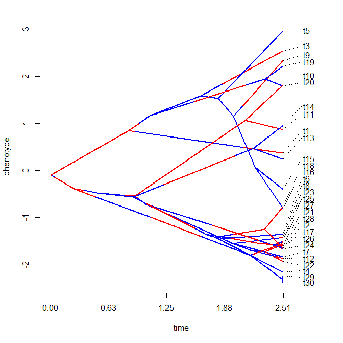
OK, now for something more interesting let's simulate a discrete character on the tree; and then generate data for two continuous traits in which both the rate & evolutionary correlation differ depending on the mapped discrete character:

> Q<-0.5*matrix(c(-1,1,1,-1),2,2)
> rownames(Q)<-colnames(Q)<-letters[1:2]
> mtree<-sim.history(tree,Q,anc="a")
> # here's our discrete character history on the tree
> plotSimmap(mtree,colors=cols,pts=F)>

> # this is for simulation
> R<-list(matrix(c(0.5,0.45,0.45,0.5),2,2),
+ matrix(c(2,0,0,2),2,2))
> names(R)<-letters[1:2]
> X<-sim.corrs(mtree,R)
> cols<-c("blue","red"); names(cols)<-letters[1:2]
> phylomorphospace(mtree,X,xlab="X1",ylab="X1",colors=cols)

Pretty cool, I guess.... The evolutionary pattern that we simulated - low rate & high evolutionary correlation on the blue branches; & high rate but low evolutionary correlation on the red branches - is pretty evident in the plot.

One little note about plotting tip labels. During the re-write I noticed that I'd used the function textxy from the package 'calibrate' in place of the base graphics function text - but I'd forgotten why. Turns out textxy is a neat function that plots text labels for points with an offset that varies depending on the plot quadrant. This is perfect for a function like phylomorphospace, because it helps push the labels away from other plotted lines & points.

That's it for now.

Bug fix for make.simmap with asymmetric substitution model; new version of phytools

Yesterday I received a user report of some problems with make.simmap(...,model="ARD") when it resulted in some of the fitted transition rates being zero. This was a known (to me) issue with make.simmap, and it is because although we can compute the conditional likelihoods with this matrix no problem - when we are trying to draw waiting times from an exponential distribution to map character changes along internal branches, rexp(...,rate=0) won't evaluate. One solution to this would be to return Inf or some arbitrarily large number when the rate is 0. Instead, and for other reasons of computation, I decide to add a small number, tol=1e-08 to off-diagonal position of Q that are 0 in the MLE. (There are also other calculations that make this necessary.)

Fixing this issue turned up another more serious problem and that is that recent versions of make.simmap have been using the transpose of Q in simulating along edges for asymmetric transition models, instead of Q itself (or, alternatively, that it has been calling a row index instead of a column index during an important stage in calculation). I believe that this bug appeared during my recent major re-write of make.simmap. Obviously, this doesn't affect symmetrical models of character change in which Q==t(Q) (such as model="ER" or model="SYM" - the default), but it will affect model="ARD".

Here's a little more specific detail on the error. In the internally called function smap, I had:

Q<-t(Q)

where I should not have; or, alternatively:

p<-expm(Q*tree$edge.length[j])[NN[j,1],]* L[as.character(tree$edge[j,2]),]

instead of:

p<-expm(Q*tree$edge.length[j])[,NN[j,1]]* L[as.character(tree$edge[j,2]),]

Source code for the fixed version of make.simmap is here. In this version, users can also control the value of tol by way of the optional argument, well, tol. tol is only used if any of the off-diagonal elements of Q are less than tol, which has a default value of tol=1e-08, as noted above.

This update to make.simmap is also in a new phytools package build, phytools 0.2-37, which can be installed from source.

Finally, here is a demo in which I simulate with a very low backward rate & then show what the new version of make.simmap does (instead of failing) if that backward transition rate has a MLE of 0. Note that if make.simmap seems to hang - it may be possible to resolve this by increasing tol.

> require(phytools)
Loading required package: phytools
> packageVersion("phytools")
[1] ‘0.2.37’
> tree<-pbtree(n=200,scale=1)
> Q<-matrix(c(-1,1,0.01,-0.01),2,2)
> rownames(Q)<-colnames(Q)<-letters[1:2]
> tree<-sim.history(tree,Q,anc="a")
> cols<-setNames(c("black","red"),letters[1:2])
> # this is the true character history
> plotSimmap(tree,cols,pts=F,ftype="off")

> mtrees<-make.simmap(tree,tree$states,model="ARD", nsim=100)

Warning: some elements of Q not numerically distinct from 0; setting to 1e-08

make.simmap is sampling character histories conditioned on the transition matrix
Q =
            a           b
a -0.96697341  0.96697341
b  0.00000001 -0.00000001
(estimated using likelihood);
and root node prior probabilities
pi =
  a   b
0.5 0.5

Done.

And a little reality check:

> # true history
> describe.simmap(tree)
1 tree with a mapped discrete character with states:
 a, b

tree has 26 changes between states

changes are of the following types:
  a  b
a 0 26
b 0  0

mean total time spent in each state is:
             a         b    total
raw  26.703708 18.438526 45.14223
prop  0.591546  0.408454  1.00000

> # stochastic maps
> describe.simmap(mtrees,plot=T,show.tip.label=FALSE)
100 trees with a mapped discrete character with states:
 a, b

trees have 25.48 changes between states on average

changes are of the following types:
       a,b b,a
x->y 25.48   0

mean total time spent in each state is:
              a          b    total
raw  26.2457674 18.8964671 45.14223
prop  0.5814016  0.4185984  1.00000

In the new phytools build I've also added the function getStates (which can be used to pull the states at nodes or tips from a tree with a mapped discrete character and is called internally by describe.simmap) to the NAMESPACE so that it can be called by phytools users.

Please don't hesitate to report any bugs or issues with the present version of make.simmap or phytools.

Thanks!