New phytools version (phytools 0.2-25)

I just posted a new minor phytools release, phytools 0.2-25, that can be downloaded and installed from source.

> install.packages("phytools_0.2-25.tar.gz",type="source", repos=NULL)
* installing *source* package 'phytools' ...
** R
...
* DONE (phytools)

This package version contains a few new functions relative to the last minor phytools build (e.g., 1, 2), along with updates to some others including (most significantly) the phytools 'traitgram' function, phenogram.

Check it out - and please post any bugs or issues.

Investigating whether the rate of one continuous trait is influenced by the state of another (a somewhat ad hoc approach)

Yesterday, the following query was submitted to the R-SIG-phylo email listserve:

I have a continuous dependent variable (e.g. range size) and a few "independent" variables (e.g. body mass, encephalization ratio), and I want to test how the rate of evolution of the dependent variable is affected by the independent variables. The PCMs that I'm familiar with cannot be used to answer this question, because they usually try to predict the dependent variable based on the independent variables (e.g. PGLM) instead of looking at the rates of evolution.

Ideally, we'd take a model-based approach to this problem, as pointed out by Matt Pennell. Unfortunately, this has not yet been done. In its stead, however, it is not too difficult to devise a somewhat ad hoc, simulation-based alternative. Here was my proposal:

What about the admittedly ad hoc approach of computing the correlation between the states at ancestral nodes for x & the squared contrasts for corresponding nodes for y? Then you can generate a null distribution for the test statistic (say, a Pearson or Spearman rank correlation) by simulation. This seems to give reasonable type I error when the null is correct, and when I simulate under the alternative (i.e., the rate of Brownian evolution along a branch depends on the state at the originating node) it sometimes is significant.

Here is the function I proposed and submitted to the list to do this, I have since posted a more sophisticated method & function here.

ratebystate<-function(tree,x,y,nsim=100,method=c("pearson","spearman")){
   method<-method[1]
   if(!is.binary.tree(tree)) tree<-multi2di(tree)
   V<-phyl.vcv(cbind(x,y),vcv(tree),lambda=1)$R
   a<-fastAnc(tree,x)
   b<-pic(y,tree)[names(a)]^2
   r<-cor(a,b,method=method)
   beta<-setNames(lm(b~a)$coefficients[2],NULL)
   foo<-function(tree,V){
      XY<-sim.corrs(tree,V)
      a<-fastAnc(tree,XY[,1])
      b<-pic(XY[,2],tree)[names(a)]^2
      r<-cor(a,b,method=method)
      return(r)
   }
   r.null<-c(r,replicate(nsim-1,foo(tree,V)))
   P<-mean(abs(r.null)>=abs(r))
   return(list(beta=beta,r=r,P=P,method=method))
}

I was naturally somewhat curious about how it would do. To figure that out, we need to simulate under the null & alternative models. The null model is trivial, of course - constant-rate Brownian motion. The alternative model is a little trickier. Here, I see two different alternatives: (1) the rate of branches descended from each internal node is a linear function of the state at that node; or (2) the rate of each branch is a linear function of the average state along that edge, where we compute the average as the mean of the rootward and tipwards nodes subtending the edge. [**Note that in the simple function above, we explicitly assume (1); however in the full version I allow for either model to be assumed using method="by.node" for (1), and method="by.branch" for (2).]

Let's first simulate under the proposed alternative model and see if the result is reasonable. I will show option (2) here:

> require(phytools)
> # simulate tree
> tree<-pbtree(n=200,scale=1)
> # simulate continuous independent variable
> x<-fastBM(tree,internal=TRUE)
> # now *scale* the branch lengths of the tree
> # by the mean of x for each edge
> ss<-rowMeans(matrix(x[tree$edge],nrow(tree$edge),2))
> zz<-tree; zz$edge.length<-zz$edge.length*(ss-min(ss))
> # visualize the scaled tree by trait relationship
> phenogram(zz,x,type="b",color="blue",ftype="off", xlab="expected variance",ylab="independent variable (x)")

> # now simulate y
> y<-fastBM(zz)
> # now let's fit our model
> source("ratebystate.R")
> ratebystate(tree,x[tree$tip.label],y,method="by.branch")
$beta
[1] 1.169129
$r
[1] 0.3187849
$P
[1] 0.01
$corr
[1] "pearson"
$method
[1] "by.branch"

Well, one simulation test does not a new method make. Here's some code that I used to run simulations under the null & alternative models [actually here under model (1), from above]:

# simulate under the null
f.null<-function(){
  tree<-pbtree(n=100)
  x<-fastBM(tree)
  y<-fastBM(tree)
  ratebystate(tree,x,y,message=FALSE)
}
sim.null<-t(replicate(400,f.null()))

# simulate under the alternative (model 1)
f.alt<-function(){
  tree<-pbtree(n=100)
  x<-fastBM(tree,internal=TRUE)
  nodes<-x[1:tree$Nnode+length(tree$tip.label)]
  zz<-tree; zz$edge.length<-zz$edge.length*(nodes[as.character(tree$edge[,1])]-min(nodes))
  y<-fastBM(zz)
  ratebystate(tree,x[tree$tip.label],y,message=FALSE)
}
sim.alt<-t(replicate(400,f.alt()))

And here are the results:

> colMeans(sim.null)
      beta           r           P
0.006199303 0.004057295 0.516675000
> mean(sim.null[,"P"]<0.05)
[1] 0.03
> colMeans(sim.alt)
    beta         r         P
1.0114919 0.2617357 0.0742000
> mean(sim.alt[,"P"]<0.05)
[1] 0.6775

So it would seem (based on these very limited simulations) that the method has type I error near or below the nominal level. Furthermore, the power is not too bad when the alternative hypothesis is correct. Finally - the mean slope of the regression between contrasts variance and ancestral states is actually very close to our generating relationship - in this case 1.0.

That's it.

Neat new function to color branches by trait value

I had a user request yesterday for a function that would plot edge colors by probability - for example, if we have a value on [0, 1] for each edge in the tree - how do we use a built-in color palette in R to plot the tree using these edges as our colors? I think that the idea is somewhat akin to what contMap or densityMap accomplish; however if all we want is to plot each edge a different color, the 'ape' function plot.phylo is just fine at doing that.

I wrote a new function, plotBranchbyTrait, which automates this - calling plot.phylo internally; but the central piece of code used by the function is relatively simple. It merely takes our probabilities or reconstructed trait values along branches of the tree and translates them to colors from a palette as follows (using, in this case, a blue→red color map):

cols<-rainbow(1000,start=0.7,end=0) # blue->red
if(is.null(xlims)) xlims<-range(x)+c(-tol,tol)
breaks<-0:1000/1000*(xlims[2]-xlims[1])+xlims[1]
whichColor<-function(p,cols,breaks){
  i<-1
  while(p>=breaks[i]&&p>breaks[i+1]) i<-i+1
  cols[i]
}
colors<-sapply(x,whichColor,cols=cols,breaks=breaks)

What we come out with is a vector of colors to use as input in the argument plot.phylo.

I also have another internally called function, add.color.map, which takes user input for location and then plots a translation map (that also serves as a scale bar, as in, for instance, densityMap). I'd never done this before, but getting an interactively user supplied position for the color map was pretty easy. Here is the code snippet that I used:

cat("Click where you want to draw the bar\n")
x<-unlist(locator(1))
y<-x[2]
x<-x[1]

This is based on something similar in the ape function add.scale.bar.

One warning to the user - the function hangs before printing the "Click where you want to draw the bar" and waits for you to supply the location before the prompt! Not sure how to fix this.

The function has three different modes. mode="edges" uses the user supplied trait value for all the edges in the tree. The input values should be in the row order of tree$edge. mode="tips" just takes tip values and it reconstructs ancestral states by using fastAnc to compute the ancestral node states, and the averages the tipward and rootward states for each edge to get the plotted color. mode="nodes" does the same averaging, but the tip and node values are user supplied.

Here's a quick and dirty demo:

> source("plotBranchbyTrait.R") # load source
> # simplest use: ancestral BM values
> tree<-pbtree(n=40)
> x<-fastBM(tree)
> plotBranchbyTrait(tree,x,method="tips")
Click where you want to draw the bar

> # now let's say we have probabilities for each edge
> pp<-fastBM(tree,bounds=c(0,1),internal=TRUE)
> p<-rowMeans(matrix(pp[tree$edge],nrow(tree$edge),2))
> plotBranchbyTrait(tree,p,xlims=c(0,1),palette="gray")
Click where you want to draw the bar

Other methods in this function should be fairly self explanatory, I hope.

That's it.

Significant update to phenogram

The phytools function phenogram does a projection of the phylogeny into a space defined by time since the root (on the x axis) and phenotype (on y). It has some nice features, for instance it can map the state of a discrete character on the tree, but it also had a couple of small bugs associated with labeling the leaves - specifically, the alignment of tip labels is messed up, and it sometimes did not leave enough whitespace right of the tips for labels to be printed.

I decided to do a significant overhaul of phenogram to both try and fix these issues as well as to enable a lot more user control of plotting within the function.

Fixing the text alignment was a piece of cake; however allocating enough whitespace for plotting tip labels turned out to be a much more complicated issue. This is not something that I've really dealt with in tree plotting before because in my other major tree plotting function, plotSimmap, the function circumvents the issue by fixing the plotting area to a unit in length, and then fractioning that area into a part for the tree and a second part for tip labels. (This works really well, but introduces complications when you want to include a legend - e.g., here.)

Let me try to explain why this (probably) seemingly trivial issue can be such a pain in the butt. Now, we have a function strwidth which will give us the width (in various units) of a plotted string. The difficulty arises if we want to tie the limits of a plotting area to a call of strwidth. This is because strwidth(...,units="user") (the default) will only work properly after our plotting device has been opened. This means that it can't be used to specify the dimensions of the plotting area - paradoxical if the point of specifying a specific set of dimensions for plotting is specifically to leave space for plotted strings! The solution* turns out to be first pull the horizontal dimension in inches of our plotting device out using par("pin"); then finding the maximum width of our tip labels (again, in inches) on the plotting devices; and then, finally, using numerical optimization to find the ratio of our units (time since the root, in this case) and inches that allows us to use the whole plotting devices when the tip labels are also plotted. The way this looks in practice is as follows:

# node heights
H<-nodeHeights(tree)
# width of the plotting device, in inches
pp<-par("pin")[1]
# string width on the plotting device, in inches
# (includes label offset)
sw<-fsize*(max(strwidth(tree$tip.label,units="inches")))+   offset*fsize*max(strwidth(tree$tip.label,
  units="inches"))/max(nchar(tree$tip.label))
# find the ratio of inches:units that fills the
# plotting window
alp<-optimize(function(a,H,sw,pp)
  (a*1.04*max(H)+sw-pp)^2,
  H=H,sw=sw,pp=pp,interval=c(0,1e6))$minimum
# set x-limits
xlim<-c(min(H),max(H)+sw/alp)

(*This solution is derived from something that Emmanuel Paradis did in the ape function plot.phylo. Thanks Emmanuel!)

While I was at it, I decided to migrate a lot of other controls over plotting to the user. This will be in the function documentation for the next phytools version, but here's a quick demo:

> source("phenogram.R")
> tree<-pbtree(n=20)
> x<-exp(fastBM(tree))
> phenogram(tree,x,log="y",colors="blue",type="b", offset=0.5,xlab="millions of years",ylab="body size", main="Body Size Evolution")

The source code for the new version of phenogram is here. It will also be updated in the next version of phytools.

New version of plotSimmap (& plotTree) for plotting leftward facing phylogenies

I was working on fixing some bugs in the phytools function phenogram when I suddenly realized how easy it would be to add left-direction plotted trees to the function plotSimmap. We do this with two simple switches. First, when we open a new plotting window we make the x-axis a "reverse axis" by reversing the vector xlim (i.e., such that xlim[1]>xlim[2]). This, without any further changes to the code, will flip all the branches of the tree to run right-to-left. Next, we change the position of the plotted text relative to the end of each leaf in the tree. In a rightward plotted tree, we want this text to be left-aligned and begin where each terminus ends running rightward. A leftward plotted tree needs right-aligned text pointing leftward. This can be changed using the text argument pos, i.e.:

pos<-if(direction=="leftwards") 2 else 4

where 2 and 4 indicate that text should be added to the left of or to the right of the plotting coordinate, respectively.

The updated code for plotSimmap is here. The following is a quick a demo of the new version in action:

> require(phytools)
> source("plotSimmap.R")
> Q<-matrix(c(-1,1,1,-1),2,2)
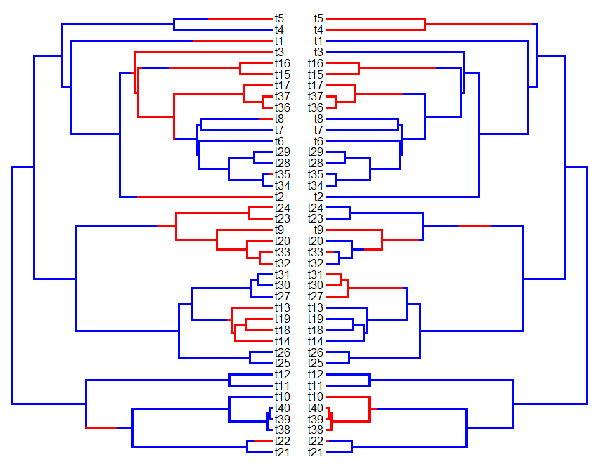
> tree<-sim.history(pbtree(n=40,scale=1),Q,nsim=2)
> cols<-c("blue","red"); names(cols)<-c(1,2)
> layout(matrix(c(1,2),1,2))
> plotSimmap(tree[[1]],cols,direction="rightwards",lwd=3, pts=F)
> plotSimmap(tree[[2]],cols,direction="leftwards",lwd=3, pts=F)

One known issue is that plotSimmap(...,direction="leftwards",node.numbers=T) doesn't work. This appears to be because the 'graphics' function symbols, which called internally to plot rectangles around each node number, doesn't seem to like a reversed x-axis. If I turn symbols off manually, i.e. just plotting text and no rectangles, the node numbers show up fine.

That's it for now.

New version of phylomorphospace with user control of x & y limits (and other things)

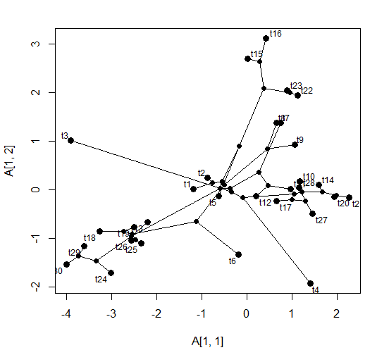
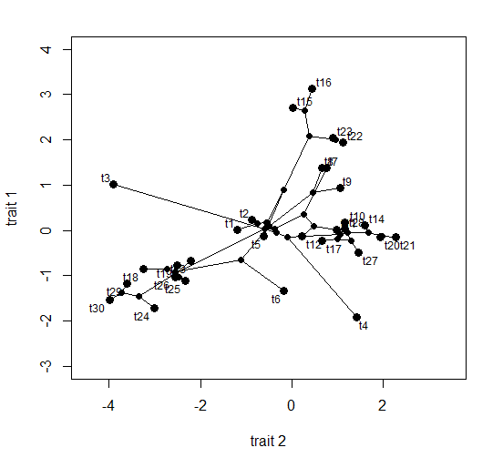
A phytools user today requested user control of x and y limits in phylomorphospace. Currently phylomorphospace sets xlim and ylim based on the range of tip and ancestral values for x & y and this can't be adjusted. It is straightforward to migrate control of this to the user, and I've done this through the "three-dot argument" (i.e., ...). I've also added user control of xlab and ylab, as well as fsize to control the font size of tip labels. fsize is relative to the default font size of textxy(...,cx=0.75).

Code for the new version of phylomorphospace is here, but because the function calls textxy in the 'calibrate' package internally, and phytools imports from calibrate, users will need to either load calibrate to run phylomorphospace from source, or they can install the newest minor build of phytools (phytools 0.2-24).

Here's a quick demo:

> require(phytools)
Loading required package: phytools
...
> packageVersion("phytools")
[1] ‘0.2.24’
> tree<-pbtree(n=30)
> XX<-fastBM(tree,nsim=2)
> par(mar=c(5.1,4.1,2.1,2.1))
> phylomorphospace(tree,XX) # default

> phylomorphospace(tree,XX,ylim=c(-3,4),xlim=c(-4.5,3.5), ylab="trait 1",xlab="trait 2")

That's it.

New version of matchNodes; new minor phytools version

I just made a couple of small updates to matchNodes (1, 2). I wrote this function primarily to be called internally by fastAnc, for which it works just fine, but I've since been frustrated when trying to use it in any task for which it wasn't originally purposed.

More specifically, the function is designed to match nodes between trees that are identical (to some measure of numerical precision) in species, topology, and possibly branch lengths (depending on method). When I tried to use it to match nodes across trees that were identical in core structure, but had different tips added, the function broke down.

The new version should (hopefully) fix this problem. Now, if trees 1 & 2 contains taxa A, B, ..., N, but tree 1 also contains taxa Q, R, S, while tree 2 contains extra taxa T, U, V, the function (using method="distances") should be able to overcome this difference and match corresponding nodes across trees.

Here's a quick demo of what I mean:

> tree<-pbtree(n=10)
> a<-add.random(tree,tips=paste("t",11:15,sep=""))
> b<-add.random(tree,tips=paste("t",16:20,sep=""))
> layout(c(1,2))
> plotTree(a,node.numbers=T)
> plotTree(b,node.numbers=T)

> matchNodes(a,b,"distances")
     tr1 tr2
[1,]  16  16
[2,]  17  NA
[3,]  18  17
[4,]  19  NA
[5,]  20  18
[6,]  21  NA
[7,]  22  19
[8,]  23  20
[9,]  24  21
[10,]  25  NA
[11,]  26  22
[12,]  27  23
[13,]  28  NA
[14,]  29  25
> matchNodes(b,a,"distances")
     tr1 tr2
[1,]  16  16
[2,]  17  18
[3,]  18  20
[4,]  19  22
[5,]  20  23
[6,]  21  24
[7,]  22  26
[8,]  23  27
[9,]  24  NA
[10,]  25  29
[11,]  26  NA
[12,]  27  NA
[13,]  28  NA
[14,]  29  NA

Inspection of these matrices, and the original trees, should show that matchNodes(a,b,"distances") gives the nodes of b (in column 2) that match each node in a; whereas matchNodes(b,a,"distances") gives the reverse.

One little nuance of this method is that we should probably allow it to tolerate inexact matches. This is because adding new edges to the tree, particularly if we then write and read the tree to and from file, will introduce random error to the distances between species and nodes - just because of rounding of branch lengths due to numerical precision of your computer or your file output format specifications. matchNodes has an argument for that: the optional argument, tol. Let's try rounding the branch lengths of each tree, examine the consequences, and then see if it can be fixed by increasing tol:

> a$edge.length<-round(a$edge.length,4)
> b$edge.length<-round(b$edge.length,4)
> matchNodes(a,b,"distances")
     tr1 tr2
[1,]  16  NA
[2,]  17  NA
[3,]  18  NA
[4,]  19  NA
[5,]  20  NA
[6,]  21  NA
[7,]  22  NA
[8,]  23  NA
[9,]  24  NA
[10,]  25  NA
[11,]  26  NA
[12,]  27  NA
[13,]  28  NA
[14,]  29  NA
> # uh-oh!!
> matchNodes(a,b,"distances",tol=0.001)
     tr1 tr2
[1,]  16  16
[2,]  17  NA
[3,]  18  17
[4,]  19  NA
[5,]  20  18
[6,]  21  NA
[7,]  22  19
[8,]  23  20
[9,]  24  21
[10,]  25  NA
[11,]  26  22
[12,]  27  23
[13,]  28  NA
[14,]  29  25

Well, that's pretty cool.

The updated function is here, but it is also in a new minor release of phytools (phytools 0.2-23), along with the new function countSimmap.