Updates to phylomorphospace3d & locate.yeti; new version of phytools

I just posted a new version of phytools. This can be downloaded from the phytools page & installed from source; however I have also submitted this version (phytools 0.4-20) to CRAN, so hopefully it will be accepted by the CRAN gatekeepers and spread out onto all the CRAN mirrors within a few days.

Some important updates in this version relative to the latest minor version include:

1. An update to locate.yeti to permit the use of a set of edge constraints to search for the ML position of the leaf to be added to the tree.

2. An update to phylomorphospace3d so that it now checks internally to see if the package rgl has been installed, and then loads it if available. This permits me to change phytools relationship with rgl from Depends to Suggests, which is designed to allow users to install & load phytools on systems where rgl cannot be installed.

This version of phytools also has a wide range of other new functions & updates relative to the last CRAN version, for instance:

1. A new version of contMap that permits some trait values for tip taxa to be missing from the dataset.

2. A new function, plotTree.wBars, that permits users to plot square or circular phylograms with bars instead of tip labels (e.g., 1, 2, 3).

3. A new function, setMap, to set the color-ramp for an object of class "contMap" or "densityMap"..

4. Some other useful updates to contMap and densityMap.

5. A new version of fancyTree that fixes a small bug for type = "scattergram".

6. The aforementioned new function (locate.yeti) for locating the position of a cryptic or recently extinct taxon on an ultrametric phylogeny using continuous character data.

7. An S3 generic method rep for objects of class "phylo" and "multiPhylo" (here).

8. A new option in phylomorphospace3d to color internal edges.

Finally, 9. New options for node placement in square phylograms plotted with plotSimmap and plotTree.

That's it!

Alternative node placements in plotted trees using plotTree & plotSimmap

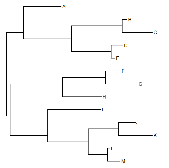
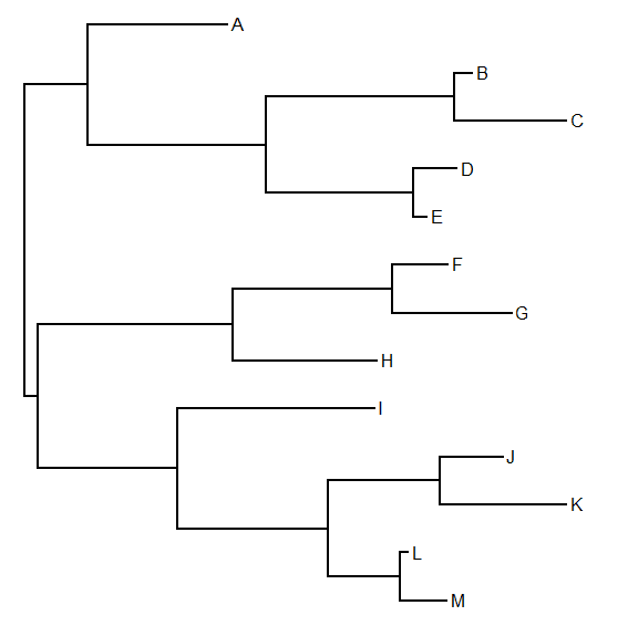
Felsenstein (2004; pp. 574-576) gives four different node placements for square phylograms. The most commonly used node placement what Felsenstein calls intermediate, i.e., the node is placed at the midpoint of the uppermost & lowermost edges immediately descended from that node. This is what that looks like for a stochastic 13 taxon tree:

> packageVersion("phytools")
[1] ‘0.4.16’
> plotTree(tree)

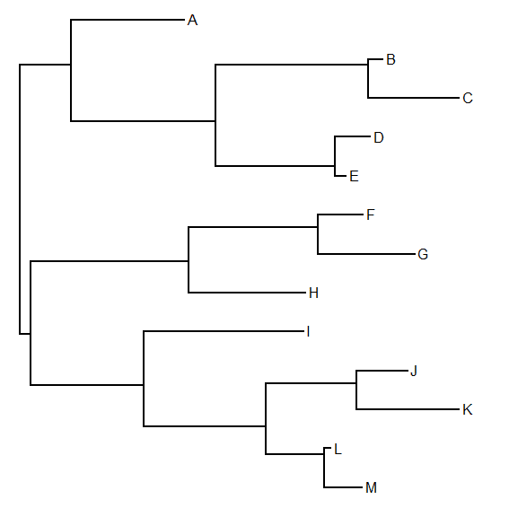
Centered node placement puts the node - instead of at the vertical point intermediate between the upper & lowermost immediate daughters - at the midpoint of all tips descended from a node. This is just the average of the upper and lowermost of this set. Here's what that looks like for the same tree:

> plotTree(tree,nodes="centered")

Like intermediate node placement, weighted node placement uses only the immediate descendants - but it weights their vertical position (inversely) by the edge length leading to each daughter node. E.g.:

> plotTree(tree,nodes="weighted")

(Note that Figure 34.1c in Felsenstein appears to use a slightly different algorithm than that described in the text - which I have followed here - in which internal and tip edges are treated differently.)

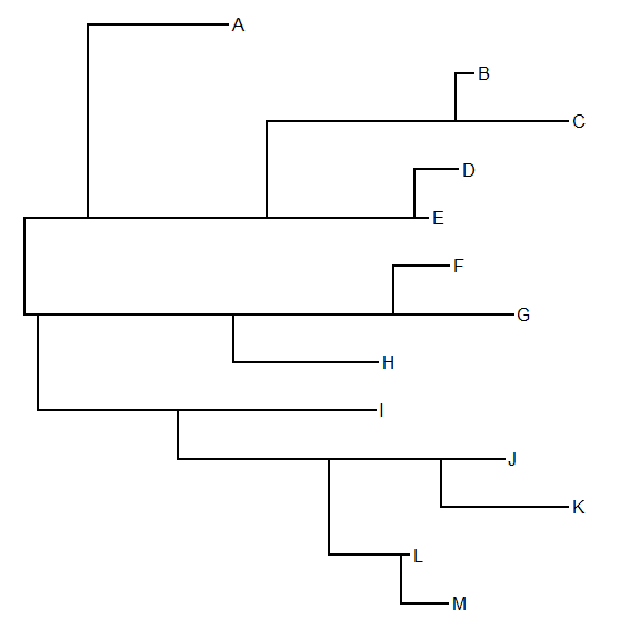
Finally, inner node placement, puts each node in the 'innermost' position of all its descendants. E.g.:

> plotTree(tree,nodes="inner")

(In this case the algorithm described by Felsenstein (2004; p. 575) seems to be incorrect unless I've misread. I achieved the desired effect not by using the of the y values of the descendant edges; but the vertical position closest to the median vertical position of all the tips.)

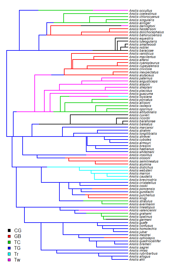
All of these methods can also be used with stochastic mapped trees (since plotSimmap is the engine that runs plotTree). For instance:

> data(anoletree)
> plotSimmap(anoletree,nodes="inner",fsize=0.7,ftype="i")
no colors provided. using the following legend:
     CG    GB       TC     TG     Tr        Tw
"black" "red" "green3" "blue" "cyan" "magenta"
> add.simmap.legend(colors=setNames(palette()[1:6],
  sort(unique(getStates(anoletree,"tips")))))
Click where you want to draw the legend

\

That's it. See some of you at 'Evolution' in a few days.

Computing the average trait value for the set of taxa descended from each node

A recent comment asked if there was an easy way to substitute the raw average value of the tips descended from a node for ancestral states obtained via ancestral state reconstruction when using the phytools function plotBranchbyTrait. This is pretty easy. Here's a demo (although it could be done a dozen different ways, including using a simple for loop).

(This assumes only that our tree is an object of class "phylo" called tree; and, importantly, that our trait data is a named vector x, in which the names correspond to the tip labels of tree.)

getDescendants<-phytools:::getDescendants
nn<-1:tree$Nnode+Ntip(tree)
a<-setNames(sapply(nn,function(n,x,t){
  d<-getDescendants(t,n)
  mean(x[t$tip.label[d[d<=Ntip(t)]]])
  },x=x,t=tree),nn)

Now we can use it with plotBranchbyTrait as follows. First, if we want each edge to be colored as the average of the parent & daughter nodes (or tip):

plotBranchbyTrait(tree,c(x,a),mode="nodes")

Alternatively, we can have the branch color determined only from the daughter nodes or tips (in which case we throw out the root value):

y<-c(setNames(x[tree$tip.label],1:Ntip(tree)),a)
plotBranchbyTrait(tree,y[tree$edge[,2]],mode="edges")

That's pretty much it.

Constraining internal node values using make.simmap

A phytools user asked the following question:

"I know I can constrain the state of the root node, but is it possible to also constrain the state at specific internal nodes?"

This is possible, although it requires a hack. We can basically attach a terminal edge (a tip) of zero length to any of the nodes that we want to constrain. We can then assign a values to that tip that is the value to which we want to constrain that node. After we conduct our stochastic mapping, we can then prune all the zero length terminal edges we've added from our stochastically mapped trees.

Here is a quick demo:

> ## first let's simulate a true character history
> tree<-pbtree(n=26,tip.label=LETTERS,scale=1)
> Q<-matrix(c(-2,2,2,-2),2,2)
> rownames(Q)<-colnames(Q)<-letters[1:2]
> true.history<-sim.history(tree,Q)
> cols<-setNames(c("blue","red"),letters[1:2])
> plotSimmap(true.history,cols)
> nodelabels()

> ## now let's run our analysis as normal
> ## (i.e., without constraint)
> x<-getStates(true.history,"tips")
> trees<-make.simmap(tree,x,nsim=100)
make.simmap is sampling character histories conditioned on the transition matrix
Q =
         a        b
a -2.29596  2.29596
b  2.29596 -2.29596
(estimated using likelihood);
and (mean) root node prior probabilities
pi =
  a   b
0.5 0.5
Done.
> ## now let's summarize the posterior probabilities
> ## at each node
> plotSimmap(trees[[1]],cols) ## one of our maps
> obj<-describe.simmap(trees)
> nodelabels(pie=obj$ace,piecol=cols,cex=0.6)

> ## next let's constrain, say, node 46 to be
> ## its true value
> x<-c(getStates(true.history,"tips"),
getStates(true.history,"nodes")["46"])
> tt<-bind.tip(tree,"46",edge.length=0,where=46)
> plotTree(tt)

> trees<-make.simmap(tt,x,nsim=100)
make.simmap is sampling character histories conditioned on the transition matrix
Q =
          a         b
a -2.219295  2.219295
b  2.219295 -2.219295
(estimated using likelihood);
and (mean) root node prior probabilities
pi =
  a   b
0.5 0.5
Done.
> ## now drop all tips "46" from the trees
> trees<-lapply(trees,drop.tip.simmap,tip="46")
> class(trees)<-"multiPhylo"
> ## now let's once again summarize our results:
> plotSimmap(trees[[1]],cols) ## one of our maps
> obj<-describe.simmap(trees)
> nodelabels(pie=obj$ace,piecol=cols,cex=0.6)

If we want to fix multiple nodes, we have to keep in mind that the node numbering will change every time that we add a tip to the tree.

In the most extreme case we might know the states at each internal node of the tree. In this case, we are just sampling reconstructions of the character history conditioned on the true (known) states at all internal nodes. This is what that might look like:

> ## pull our data vector
> x<-c(getStates(true.history,"tips"),
getStates(true.history,"nodes"))
> nodes<-1:tree$Nnode+length(tree$tip.label)
> for(i in 1:length(nodes)){
if(i==1) tt<-bind.tip(tree,nodes[i],where=nodes[i],edge.length=0)
else {
M<-matchNodes(tree,tt)
tt<-bind.tip(tt,nodes[i],where=M[which(M[,1]==nodes[i]),2],
edge.length=0)
}
}
> plotTree(tt)

> ## now run stochastic mapping
> trees<-make.simmap(tt,x,nsim=100)
make.simmap is sampling character histories conditioned on the transition matrix
Q =
a b
a -2.91958 2.91958
b 2.91958 -2.91958
(estimated using likelihood);
and (mean) root node prior probabilities
pi =
a b
0.5 0.5
Done.
> ## drop all added tips
> trees<-lapply(trees,drop.tip.simmap,
tip=as.character(nodes))
> class(trees)<-"multiPhylo"
> ## visualize the results
> plotSimmap(trees[[1]],cols) ## one of our maps
> obj<-describe.simmap(trees)
> nodelabels(pie=obj$ace,piecol=cols,cex=0.6)

We can even do the following:

> obj<-densityMap(trees,plot=FALSE)
sorry - this might take a while; please be patient
> plot(obj,lwd=4,outline=TRUE)

Which, in this case, shows the uncertainty about where transitions between states occurred, even when conditioned on knowing the true states at all nodes.

Finally, since make.simmap also allows us to supply a prior on tip states, we can use the same hack to put a prior on internal nodes.

OK. That's it for now.

Coloring edges in phylomorphospace3d

A recent R-sig-phylo query asked the following about phytools function phylomorphospace3d (for projecting a tree into a three-dimensional morphospace):

"[Is t]here is a possbility to color some specific edges in the phylomorphospace3d()? plot.phylo() has the argument "edge.color" to do that in classical tree plotting. I need it, however, in the above mentioned function."

This functionality (as well as the ability to plot a stochastic character map on a phylomorphospace) exists for two-dimensional phylomorphospace plotting, but it did not (until now) exist for phylomorphospace3d; however, this was not too difficult to add. I have added user control of plotted line colors via the control parameter col.edge (as in phylomorphospace), rather than via a new function argument.

Code for this new function version is here; but users may prefer to install the latest bleeding edge source version of phytools (phytools 0.4-14) to ensure that everything works as advertised.

Here is a demo that plots the internal edges of a 3D phylomorphospace in blue, while the terminal edges are plotted in red:

## load phytools
require(phytools)
packageVersion("phytools") ## should be >=0.4-14
## simulate tree
tree<-pbtree(n=12,tip.label=LETTERS[1:12])
X<-fastBM(tree,nsim=3)
## create color vector
colors<-sapply(tree$edge[,2], function(x,n) if(x>n) "blue"
  else "red",n=length(tree$tip.label))
## generate 3D phylomorphospace plot
phylomorphospace3d(tree,X,control=list(lwd=2,
  col.edge=colors))

BTW, to create this cool .gif, you just need to do something like:

movie3d(phylomorphospace3d(tree,X,control=list(lwd=2,
  col.edge=colors)),movie="phylomorph-3d",duration=10)

The same option is also available for method="static", e.g.:

phylomorphospace3d(tree,X,control=list(lwd=2,
  col.edge=colors),method="static",angle=20)

That's it.

Performing stepwise phylogenetic regression in R

A colleague asked the following:

"Is there a way to do a multiple stepwise regression on continuous data that incorporates phylogenetic information and selects the best model based on an AICc score?"

Although I myself had not done this before, I figured that stepwise regression with objects of class "gls" would likely be something that someone, somewhere, in the wide world of R would have thought of before - and this is indeed correct.

Here's a complete demo with simulation code.

First, simulate data. In this case, x₁ and x₃ have an effect on y, so they ought to be found in the final model - but x₂ and x₄ intentionally do not.

## load packages
require(phytools)
require(nlme)
require(MASS)

## simulate data (using phytools)
tree<-pbtree(n=26,tip.label=LETTERS)
x1<-fastBM(tree)
x2<-fastBM(tree)
x3<-fastBM(tree)
x4<-fastBM(tree)
y<-0.75*x1-0.5*x3+fastBM(tree,sig2=0.2)
X<-data.frame(y,x1,x2,x3,x4)

Now let's fit our model & run the stepwise regression method using AIC:

## build model (using nlme)
obj<-gls(y~x1+x2+x3+x4,data=X,correlation=
  corBrownian(1,tree),method="ML")

## run stepwise AIC (using MASS & nlme)
fit<-stepAIC(obj,direction="both",trace=0)

trace just controls the amount of information about the backward & forward stepwise procedure that is being run. If we want more, we should increase it.

Finally, here's a worked simulation with results:

> ## simulate data (using phytools)
> tree<-pbtree(n=26,tip.label=LETTERS)
> x1<-fastBM(tree)
> x2<-fastBM(tree)
> x3<-fastBM(tree)
> x4<-fastBM(tree)
> y<-0.75*x1-0.5*x3+fastBM(tree,sig2=0.2)
> X<-data.frame(y,x1,x2,x3,x4)
> ## build model (using nlme)
> obj<-gls(y~x1+x2+x3+x4,data=X,correlation=
  corBrownian(1,tree),method="ML")
> ## run stepwise AIC (using MASS & nlme)
> fit<-stepAIC(obj,direction="both",trace=0)
> fit
Generalized least squares fit by maximum likelihood
  Model: y ~ x1 + x3
  Data: X
  Log-likelihood: -10.43514

Coefficients:
(Intercept)          x1          x3
-0.4952197   0.6882657  -0.5108970

Correlation Structure: corBrownian
Formula: ~1
Parameter estimate(s):
numeric(0)
Degrees of freedom: 26 total; 23 residual
Residual standard error: 0.594681

This is just about what we'd expect. Cool.

Generic rep (replicate) function for objects of class "phylo" & "multiPhylo"

Again, working on something else, I realized that there is no generic rep (replicate elements of vectors or lists) function for objects of class "phylo" or "multiPhylo". These were straightforward to do (although undoubtedly could've been programmed more elegantly & they use c.phylo & c.multiPhylo. The only hitch was in appending an additional tree to a list (object of class "multiPhylo"), we can't use c.multiPhylo without doing:

obj<-c(obj,list(x))

Here is the code:

rep.phylo<-function(x,...){
  if(hasArg(times)) times<-list(...)$times
  else times<-(...)[[1]]
  for(i in 1:times)
    obj<-if(i==1) x else if(i==2) c(obj,x) else
      c(obj,list(x))
  class(obj)<-"multiPhylo"
  obj
}

rep.multiPhylo<-function(x,...){
  if(hasArg(times)) times<-list(...)$times
  else times<-(...)[[1]]
  for(i in 1:times) obj<-if(i==1) x else if(i>=2) c(obj,x)
  class(obj)<-"multiPhylo"
  obj
}

I will add to a future version of phytools.

Plotting a slanted cladogram using phytools

I inadvertently discovered the algorithm for plotting a right-facing slanted cladogram this evening. Basically, to get the vertical position of each internal node we just assign heights 1 through N to the tips; and then each internal node is merely the simple arithmetic mean of its descendants. We get the horizontal positions (the heights above the root) using the method of Grafen with ρ=1, implemented in the ape function compute.brlen.

We can apply this algorithm via the phytools function phenogram as follows:

plotCladogram<-function(tree){
  foo<-function(tree,x){
   n<-1:tree$Nnode+length(tree$tip.label)
   setNames(sapply(n,function(n,x,t) mean(x[Descendants(t,n,
    "tips")[[1]]]),x=x,t=tree),n)
  }
  tree<-reorder(tree,"cladewise")
  x<-setNames(1:length(tree$tip.label),tree$tip.label)
  phenogram(compute.brlen(tree),c(x,foo(tree,x)),ylab="")
}

For example:

> require(phytools)
> require(phangorn)
> tree<-pbtree(n=26,tip.label=LETTERS[26:1])
> plotCladogram(tree)

Locating the phylogenetic postion of the Yeti: Placing cryptic, recently extinct, or hypothesized taxa in an ultrametric phylogeny using continuous character data

I recently returned from teaching in the AnthroTree 2014 Workshop. This is a course organized by Charlie Nunn that is designed to (in brief) introduce anthropologists to basic & advanced methods in phylogenetic comparative biology.

Well, I won't get into too many details, but a grad student in the workshop was interested in placing a hypothesized taxon into an ultrametric phylogeny when she had only continuous character data for this focal species, along with the same characters measured for all the other species in the phylogeny. This turns out to be not a very hard problem. It has the following parts:

(1) Computing the likelihood of continuous character data on a tree. This is not hard. We can just use the method of Felsenstein (1973), which is actually exactly equivalent to computing the likelihood of a Brownian motion model on our tree using standard comparative method machinery.

(2) Accounting for correlations among characters. This is important when the tree is unknown - but in this case we have a base tree containing all but one of our taxa. This makes accounting for correlations among characters in our likelihood calculation quite straightforward. We can just rotate our data using phylogenetic PCs obtained via PCA on the N - 1 tips in our base tree. We then compute the scores for all the taxa in the tree, and the taxon of unknown phylogenetic affinity. Finally, our log-likelihood just becomes the summed log-likelihoods of each of these now evolutionarily orthogonal characters.

(3) Finding the ML tree. Well, unlike the problem of ML optimization from continuous characters when the tree is unknown, this just involves - at worst - optimizing the position of the new branch along each of the 2(N - 2) edges in our base tree, and then picking the edge and position that maximized the likelihood. In reality, we can probably just compute the likelihood from the midpoint of each edge, and then narrow our search to a much smaller set of edges which we search more thoroughly. We only have to find the divergence point because our tree is ultrametric and our new taxon is (we have assumed) extant.

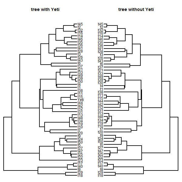
Graham Slater suggested this method be called (facetiously, of course) locate.yeti, and I have just now posted code for this on the phytools page. Here's a quick demo of just how well it works:

## load required packages
require(phytools)
require(phangorn)
require(mnormt)

## load source
source("locate.yeti.R")

## simulate tree & data
N<-50 ## taxa in base tree
m<-10 ## number of continuous characters
## simulate tree
tt<-tree<-pbtree(n=N+1,tip.label=sample(c(paste("t",1:N,
  sep=""),"Yeti")))
## generate a covariance matrix for simulation
L<-matrix(rnorm(n=m*m),m,m)
L[upper.tri(L,diag=FALSE)]<-0
L<-L-diag(diag(L))+abs(diag(diag(L)))
V<-L%*%t(L)
X<-sim.corrs(tree,vcv=V)
## visualize trees
par(mfrow=c(1,2))
plotTree(tt,mar=c(0.1,0.1,4.1,0.1))
title("tree with Yeti")
tree<-drop.tip(tree,"Yeti")
plotTree(tree,mar=c(0.1,0.1,4.1,0.1),direction="leftwards")
title("tree without Yeti")

## run locate.yeti
mltree<-locate.yeti(tree,X,plot=T)

(This plot shows the likelihood of attaching the tip to any edge.)

## plot results
par(mfrow=c(1,2))
plotTree(tt,mar=c(0.1,0.1,4.1,0.1))
title("true position of Yeti")
plotTree(mltree,mar=c(0.1,0.1,4.1,0.1),
  direction="leftwards")
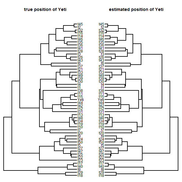
title("estimated position of Yeti")

## compute RF distance
RF.dist(tt,mltree)
## [1] 0

(Of course, it doesn't always do this well!)

In my optimization routine, I take the single edge with the highest likelihood from step one, and then get its parent (if one exists) and daughter (likewise) edges. Then I perform numerical optimization of the position of the cryptic lineage on each of these one, two, three, or more edges. Finally, I pick the edge & location with the highest likelihood. It is, of course, possible that an edge with the cryptic taxon at its midpoint might have an even higher likelihood if that taxon was placed somewhere else along the edge, so this would be the next natural step in expanding this heuristic to have better confidence that we have found the ML position.

Finally, there is no theoretical difficulty in using the same general approach to place a fossil taxon on the tree. In that case we just have one additional parameter to optimize - the terminal edge length. Similarly, we could also using a Bayesian MCMC approach to (say) put prior probabilities on the edges that are more or less likely to have produced our cryptic or fossil lineage.

That's it for now.

New version of fancyTree for type="scattergram"

I just fixed a small bug in fancyTree(...,type="scattergram") that can cause axis labels to suddenly appear inside the multi-panel plot when edited using an external application. Just as a reminder, fancyTree(...,type="scattergram") creates a type of 'phylogenetic scatterplot matrix' for two or more continuous characters & a tree:

> require(phytools)
Loading required package: phytools
> tree<-pbtree(n=26,tip.label=LETTERS[26:1])
> X<-fastBM(tree,nsim=3)
> fancyTree(tree,type="scattergram",X=X)

Code is here, and a 'bleeding-edge' phytools version with this update can be found here.

phytools blog no longer permits anonymous comments

Basically, the post title says it all. The phytools blog was getting so many spam comments (and more & more of it was getting through the automatic blogger spam filters) that it was starting to displace genuine questions & comments. Please email me if you try to comment on this blog & fail, or if you find that the new limitations on commenting are too restrictive. Thanks!