Alternative node placements in plotted trees using plotTree & plotSimmap

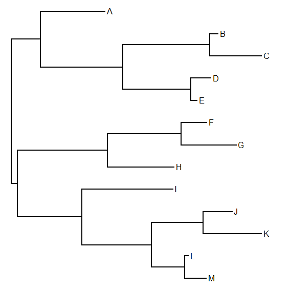
Felsenstein (2004; pp. 574-576) gives four different node placements for square phylograms. The most commonly used node placement what Felsenstein calls intermediate, i.e., the node is placed at the midpoint of the uppermost & lowermost edges immediately descended from that node. This is what that looks like for a stochastic 13 taxon tree:

> packageVersion("phytools")
[1] ‘0.4.16’
> plotTree(tree)

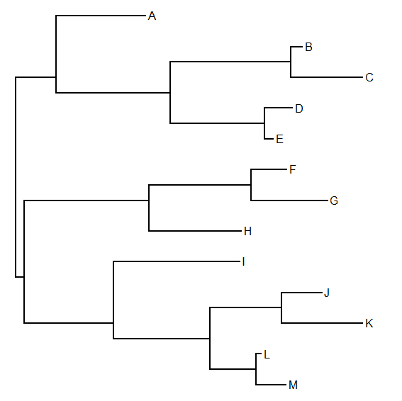
Centered node placement puts the node - instead of at the vertical point intermediate between the upper & lowermost immediate daughters - at the midpoint of all tips descended from a node. This is just the average of the upper and lowermost of this set. Here's what that looks like for the same tree:

> plotTree(tree,nodes="centered")

Like intermediate node placement, weighted node placement uses only the immediate descendants - but it weights their vertical position (inversely) by the edge length leading to each daughter node. E.g.:

> plotTree(tree,nodes="weighted")

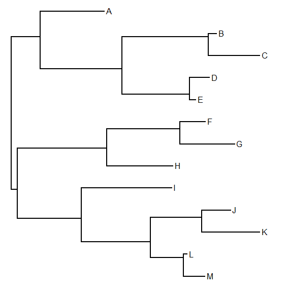
(Note that Figure 34.1c in Felsenstein appears to use a slightly different algorithm than that described in the text - which I have followed here - in which internal and tip edges are treated differently.)

Finally, inner node placement, puts each node in the 'innermost' position of all its descendants. E.g.:

> plotTree(tree,nodes="inner")

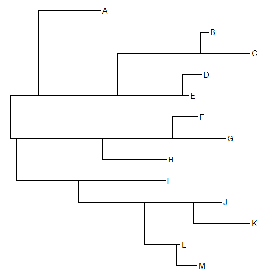
(In this case the algorithm described by Felsenstein (2004; p. 575) seems to be incorrect unless I've misread. I achieved the desired effect not by using the of the y values of the descendant edges; but the vertical position closest to the median vertical position of all the tips.)

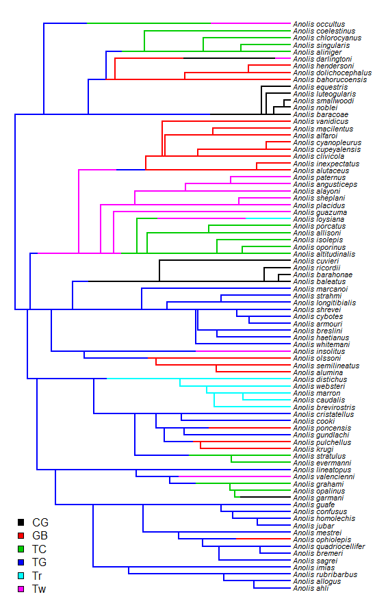
All of these methods can also be used with stochastic mapped trees (since plotSimmap is the engine that runs plotTree). For instance:

> data(anoletree)
> plotSimmap(anoletree,nodes="inner",fsize=0.7,ftype="i")
no colors provided. using the following legend:
     CG    GB       TC     TG     Tr        Tw
"black" "red" "green3" "blue" "cyan" "magenta"
> add.simmap.legend(colors=setNames(palette()[1:6],
  sort(unique(getStates(anoletree,"tips")))))
Click where you want to draw the legend

\

That's it. See some of you at 'Evolution' in a few days.