Sunday, March 31, 2013

Small update to phylosig

The following query was recently posted to the bioinformatics question & answer site, BioStar:

"I use phytools to analyse phylogenetic signal in different tree topologies. In likelihood ratio test with likelihoods for Pagel's lambda I recieve p-value=0 in all my topologies (1000 trees). Not 0.000, or something like that, just 0. I understand, that it indicates highly significant LRT result. But I'm in doubt, is it theoretically possible? And what does it mean from mathematical point of view?"

The posted answer (that is that the P-value is low enough to push the limit of its floating point representation in the method as implemented) is pretty much right on the money; however there is a little more nuance in that I for some reason have computed the P-value of the likelihood-ratio using:

1-pchisq(...)
instead of:
pchisq(...,lower.tail=FALSE)

This distinction is inconsequential until pchisq(...) approaches 1 (to a very high degree of numerical precision), at which point 1-pchisq(...) goes to 0. This can be true even if pchisq(...,lower.tail=FALSE) is numerically distinguishable from 0.

So, for instance:

> 1-pchisq(10,df=1)
[1] 0.001565402
> pchisq(10,df=1,lower.tail=FALSE)
[1] 0.001565402
> 1-pchisq(20,df=1)
[1] 7.744216e-06
> pchisq(20,df=1,lower.tail=FALSE)
[1] 7.744216e-06
> # but...
> 1-pchisq(80,df=1)
[1] 0
> pchisq(80,df=1,lower.tail=FALSE)
[1] 3.744097e-19

Does this distinction between P=3.74×10⁻¹⁹ and P=0 "matter" (that is, even ignoring the fact that the χ2 only approximates the probability distribution of the likelihood-ratio anyway)? Well, of course not. Nonetheless, this is easy enough to fix. Here's a link to the updated version. Let's load a new build of phytools containing this update and try it:

> require(phytools)
Loading required package: phytools
> packageVersion("phytools")
[1] ‘0.2.34’
> # simulate tree & data
> tree<-pbtree(n=100)
> x<-fastBM(tree)
> phylosig(tree,x,method="lambda",test=TRUE)
$lambda
[1] 1.000031
$logL
[1] -135.1252
$logL0
[1] -201.9702
$P
[1] 0

> detach("package:phytools",unload=TRUE)
> install.packages("phytools_0.2-35.tar.gz",type="source", repos=NULL)
* installing *source* package 'phytools' ...
...
* DONE (phytools)
> require(phytools)
Loading required package: phytools
> packageVersion("phytools")
[1] ‘0.2.35’
> phylosig(tree,x,method="lambda",test=TRUE)
$lambda
[1] 1.000031
$logL
[1] -135.1252
$logL0
[1] -201.9702
$P
[1] 6.387017e-31

That's it.

Random trees for a set of taxa

A phytools user recently asked:

"Is there any function in your package that can randomize the shape of a phylogeny? e.g. randomize the topology of a phylogenetic tree?

I'm going to liberally interpret this to mean - how do we simulate random trees for a set of tip taxa?

This is straightforward using the phytools function pbtree, but we could equally well substitute rtree from ape, birthdeath.tree in geiger, or any of the more flexible tree simulation functions in TreeSim; basically anything that creates an object of class "multiPhylo".

Here's how we do it:

# for our simulations, let's set...
species<-LETTERS

# simulate random trees (using any simulator)
random.trees<-pbtree(n=length(species),nsim=100)
# now apply our tip labels
random.trees<-lapply(random.trees,
   function(x,sp){ x$tip.label<-sample(sp); x },
   sp=sample(species))
class(random.trees)<-"multiPhylo"

That's it.

Saturday, March 30, 2013

Estimating ancestral states when tips are uncertain

I recently received an email with the following content (among other things):

"Have you ever considered developing algorithms for inferring character states for taxa that are missing data? I looked at phytools and did not see an application that does this."

Well, first of all, at least one method in phytools, the function ancThresh for ancestral character estimation under the threshold model, does allow for uncertain tip states by permitting input of known states or a matrix of prior probabilities on tips. In the case where data were totally unknown (i.e., missing) we would just provide a completely uninformative prior probability distribution for the state.

It is relatively straightforward to use the same general idea if sampling ancestral character histories using the method of stochastic character mapping. As discussed in prior posts (e.g., 1, 2) it is easy to get the marginal probabilities from joint sampling of ancestral states using stochastic mapping. I have posted an updated version of make.simmap that can take as input either a character state vector of a matrix of prior probabilities for tip states.

Implementation of this was surprisingly easy. First, I modified the internally called function apeAce - in which I have adapted code from ape's ace to compute the scaled conditional likelihoods for internal nodes. Here, I just need to adjust the code slightly so that we use the prior probabilities for tip states during post-order tree traversal during the pruning algorithm. Next, I modified the mapping code so that tip edges are treated the same way as internal edges. In this way we can assign node and tip states stochastically via pre-order tree traversal in the first step of the mapping algorithm described in Bollback (2006). Piece of cake!

One of the interesting features of both this method & ancThresh is that it allows us to estimate the posterior probability that uncertain tips are in any state.

Here's a quick demo. This also uses an updated version of desribe.simmap. Both updated functions are in the latest minor release of phytools (phytools 0.2-34), which can be downloaded & installed from source:

> # load phytools & dependencies
> require(phytools)
> packageVersion("phytools")
[1] ‘0.2.34’
> # this function turns a discrete character into a
> # binary matrix
> to.matrix<-function(x,seq) sapply(seq,"==",x)*1
>
> # simulate tree & data
> tree<-pbtree(n=25,scale=1)
> Q<-matrix(c(-2,1,1,1,-2,1,1,1,-2),3,3)
> rownames(Q)<-colnames(Q)<-letters[1:3]
> x<-sim.history(tree,Q)$states
> x
 t9 t10  t7 t18 t19  t1 t14 t15  t3  t8 t11 t16 t17 t13 t20
"a" "c" "c" "c" "c" "a" "b" "b" "c" "a" "c" "c" "c" "c" "b"
t21  t6  t4  t5 t24 t25 t12  t2 t22 t23
"c" "a" "c" "c" "c" "c" "c" "c" "a" "a"
> # convert to binary matrix
> PP<-to.matrix(x,letters[1:3])
> PP
    a b c
t9  1 0 0
t10 0 0 1
t7  0 0 1
t18 0 0 1
t19 0 0 1
t1  1 0 0
t14 0 1 0
t15 0 1 0
t3  0 0 1
t8  1 0 0
t11 0 0 1
t16 0 0 1
t17 0 0 1
t13 0 0 1
t20 0 1 0
t21 0 0 1
t6  1 0 0
t4  0 0 1
t5  0 0 1
t24 0 0 1
t25 0 0 1
t12 0 0 1
t2  0 0 1
t22 1 0 0
t23 1 0 0

OK now let's make some of our tip states (arbitrarily) uncertain:

> # t20 might be 'a' or 'b'
> PP["t20",2:3]<-c(0.5,0.5)
> # we are totally ignorant about t2 and t23
> PP["t2",]<-rep(1/3,3)
> PP["t23",]<-rep(1/3,3)
> PP
        a     b     c
t9  1.000 0.000 0.000
t10 0.000 0.000 1.000
t7  0.000 0.000 1.000
t18 0.000 0.000 1.000
t19 0.000 0.000 1.000
t1  1.000 0.000 0.000
t14 0.000 1.000 0.000
t15 0.000 1.000 0.000
t3  0.000 0.000 1.000
t8  1.000 0.000 0.000
t11 0.000 0.000 1.000
t16 0.000 0.000 1.000
t17 0.000 0.000 1.000
t13 0.000 0.000 1.000
t20 0.000 0.500 0.500
t21 0.000 0.000 1.000
t6  1.000 0.000 0.000
t4  0.000 0.000 1.000
t5  0.000 0.000 1.000
t24 0.000 0.000 1.000
t25 0.000 0.000 1.000
t12 0.000 0.000 1.000
t2  0.333 0.333 0.333
t22 1.000 0.000 0.000
t23 0.333 0.333 0.333

Finally, let's do stochastic character mapping (and estimate ancestral states) using either our true data, or our data with uncertainty and missing data for some tips.

> # true data
> atrees<-make.simmap(tree,x,nsim=200,model="ER")
make.simmap is sampling character histories conditioned on the transition matrix
Q =
           a          b          c
a -1.4409903  0.7204951  0.7204951
b  0.7204951 -1.4409903  0.7204951
c  0.7204951  0.7204951 -1.4409903
(estimated using likelihood);
and state frequencies (used to sample the root node following Bollback 2006)
pi =
        a         b         c
0.3333333 0.3333333 0.3333333
> # data with uncertainty
> btrees<-make.simmap(tree,PP,nsim=200,model="ER")
make.simmap is sampling character histories conditioned on the transition matrix
Q =
           a          b          c
a -1.1736451  0.5868225  0.5868225
b  0.5868225 -1.1736451  0.5868225
c  0.5868225  0.5868225 -1.1736451
(estimated using likelihood);
and state frequencies (used to sample the root node following Bollback 2006)
pi =
        a         b         c
0.3333333 0.3333333 0.3333333
> # compute posterior probabilities at nodes & tips
> AA<-describe.simmap(atrees,plot=TRUE)
200 trees with a mapped discrete character with states:
 a, b, c

trees have 14.255 changes between states on average

changes are of the following types:
      a,b  a,c   b,a  b,c  c,a  c,b
x->y 1.37 3.82 1.045 1.67 4.01 2.34

mean total time spent in each state is:
             a          b         c    total
raw  2.2430532 0.78932529 5.2821745 8.314553
prop 0.2697744 0.09493298 0.6352927 1.000000

> BB<-describe.simmap(btrees,plot=TRUE)
200 trees with a mapped discrete character with states:
 a, b, c

trees have 11.755 changes between states on average

changes are of the following types:
       a,b  a,c b,a   b,c   c,a  c,b
x->y 1.005 3.21 0.8 1.075 4.145 1.52

mean total time spent in each state is:
             a          b        c    total
raw  2.1909087 0.73316975 5.390475 8.314553
prop 0.2635029 0.08817909 0.648318 1.000000

One of the neat attributes of this approach is that in addition to estimates at internal nodes, we also get posterior probabilities for tips. These are plotted in the figure above. (The necessary downside, of course, is that sometimes these estimates will be wrong, as is the case for tip t20, which we infer with high confidence is green when it should actually be red.)

That's it.

Thursday, March 28, 2013

Marginal ancestral state reconstruction using multiple methods

Rob Lanfear asks:

"A quick question to follow up on your two posts, and some recent discussion on the R list: do you have a good feeling for the quickest implementation to do this on large trees? (Happy to assume for the purposes of this question that I'm O.K. with the stochastic variation in stochastic character mapping, and that I'm not worried about the differences between marginal frequencies and marginal probabilities...)"

I was about to submit a response to the comment directly - but then it occurred to me that other readers might be interested as well.

The fastest in R seems to be ASR using Rich Fitzjohn's package diversitree, although it is a little more difficult to use than what I have in phytools.

I did not compare, however, to phangorn, which Klaus Schliep showed us can also be used quite nicely.

Here's some demo code, including simulation, with comments:

# load packages
require(phytools)
require(diversitree)

# simulate using phytools:
tree<-pbtree(n=100,scale=1)
Q<-matrix(c(-2,1,1,1,-2,1,1,1,-2),3,3)
rownames(Q)<-colnames(Q)<-1:3
x<-sim.history(tree,Q)$states

# ASR using rerootingMethod
XX<-rerootingMethod(tree,x,model="ER")
# ASRs in XX$marginal.anc

# ASR using make.simmap
mtrees<-make.simmap(tree,x,model="ER",nsim=100)
# (we should ideally increase nsim, if possible)
YY<-describe.simmap(mtrees)
# ASRs in YY$ace

# ASR using diversitree
y<-setNames(as.numeric(x),names(x))
# (we needed to convert to numeric)
lik<-make.mkn(tree,y,k=3)
# constrain to ER model
lik<-constrain(q13~q12,q21~q12,q23~q12,q31~q12,q32~q12)
fit<-find.mle(lik,setNames(1,argnames(lik)))
ZZ<-t(asr.marginal(lik,coef(fit)))
dimnames(ZZ)<-dimnames(XX$marginal.anc)

(**Note that I'm not that experienced with diversitree, so please post corrections if the above was not done properly.)

In theory, rerootingMethod & asr.marginal should give identical estimates for any model in which all qij=qji. make.simmap will give different ancestral state estimates, but these will be highly correlated as nsim is made to be large.

Saturday, March 23, 2013

New version of describe.simmap with informative message

I just posted a new version of describe.simmap that prints an informative message and returns the results invisibly (if message is set to TRUE). This can be used on a single tree simulated with sim.history, or on a set of stochastic maps obtained using make.simmap or read in with read.simmap from the stand-alone program SIMMAP. Here's a demo:

> library(phytools)
> # simulate data
> tree<-pbtree(n=100,scale=1)
> Q<-matrix(c(-2,1,1,1,-2,1,1,1,-2),3,3)
> rownames(Q)<-colnames(Q)<-LETTERS[1:3]
> tree<-sim.history(tree,Q,anc="A")
> # conduct stochastic mapping on simulated data
> mtrees<-make.simmap(tree,tree$states,model="ER",nsim=100)
make.simmap is sampling character histories conditioned on the transition matrix
Q =
          A         B         C
A -2.304145  1.152073  1.152073
B  1.152073 -2.304145  1.152073
C  1.152073  1.152073 -2.304145
(estimated using likelihood);
and state frequencies (used to sample the root node following Bollback 2006)
pi =
        A         B         C
0.3333333 0.3333333 0.3333333

> # simulated data
> describe.simmap(tree)
1 tree with a mapped discrete character with states:
 A, B, C

tree has 42 changes between states

changes are of the following types:
  A B  C
A 0 8  6
B 3 0 11
C 9 5  0

mean total time spent in each state is:
             A         B         C    total
raw  8.2115414 5.5285739 7.9719994 21.71211
prop 0.3782009 0.2546308 0.3671683  1.00000

> # stochastic mapping results
> describe.simmap(mtrees,plot=TRUE)
100 trees with a mapped discrete character with states:
 A, B, C

trees have 55.72 changes between states on average

changes are of the following types:
      A,B  A,C  B,A   B,C  C,A  C,B
x->y 7.43 9.67 8.48 12.57 8.79 8.78

mean total time spent in each state is:
             A         B         C    total
raw  7.7147098 6.9697895 7.0276153 21.71211
prop 0.3553182 0.3210092 0.3236725  1.00000

Code is here - plus new phytools build (phytools 0.2-32) to install from source.

Friday, March 22, 2013

Bug fix for describe.simmap

There was a small bug in this new function to summarize the results of stochastic mapping that I posted yesterday, describe.simmap, for describe.simmap(...,plot=TRUE). The fixed version of this, plus updated code for the re-rooting method of ancestral state reconstruction, are on the phytools webpage. I also posted a new minor build of phytools (phytools 0.2-31) containing these updates.

Thursday, March 21, 2013

Function to summarize the results of stochastic mapping

To address a user request I just quickly wrote a new utility function, describe.simmap, to summary the results from stochastic maps on one or multiple trees. It computes the total number of transitions and the number of each type (using countSimmap; and it computes the posterior probabilities for each node. Finally it can optionally plot those probabilities on a tree. Basically, it pulls together some different things that I've been doing for analyses and visualization in some recent posts (e.g., 1, 2, 3, 4, 5, 6). Code is here.

Here's a demo:

> library(phytools)
> source("describe.simmap.R")
> tree<-pbtree(n=60,scale=1)
> Q<-matrix(c(-3,1,1,1,1,-3,1,1,1,1,-3,1,1,1,1,-3),4,4)
> rownames(Q)<-colnames(Q)<-c("a","c","g","t")
> x<-sim.history(tree,Q)$states
> mtrees<-make.simmap(tree,x,model="ER",nsim=100)
make.simmap is sampling character histories conditioned on the transition matrix
Q =
           a          c          g          t
a -2.8373734  0.9457911  0.9457911  0.9457911
c  0.9457911 -2.8373734  0.9457911  0.9457911
g  0.9457911  0.9457911 -2.8373734  0.9457911
t  0.9457911  0.9457911  0.9457911 -2.8373734
(estimated using likelihood);
and state frequencies (used to sample the root node following Bollback 2006)
pi =
   a    c    g    t
0.25 0.25 0.25 0.25
> XX<-describe.simmap(mtrees,plot=TRUE,cex=0.7)
> XX
$count
       N a,c a,g a,t c,a c,g c,t g,a g,c g,t t,a t,c t,g
 [1,] 64   4   8   6   3   5   1  12   6   5   6   3   5
 [2,] 46   4   3   2   4   5   3   9   6   4   1   3   2
 [3,] 46   4   4   0   3   3   3   4   8   5   4   3   5
 [4,] 55   7   8   3   5   7   3   5   5   1   5   5   1
 [5,] 59 ...

$ace
       a    c    g    t
61  0.20 0.31 0.31 0.18
62  0.24 0.32 0.29 0.15
63  0.12 0.87 0.00 0.01
64  0.12 0.87 0.00 0.01
65  ...

$legend
black    red green3   blue
  "a"    "c"    "g"    "t"

That's it.

A little more on ancestral state estimation

What is true of marginal ancestral state estimates is that (for a reversible model of evolution) they are equivalent to the conditional scaled likelihoods at the root node of the tree. This is stated in Felsenstein (2004), p. 259. Thus, we should be able to move the root to each node and recalculate the scaled conditional likelihoods for that node.

A simple function to do this in R is as follows:

rerootingMethod<-function(tree,x,model=c("ER","SYM")){
  model<-model[1]
  n<-length(tree$tip.label)
  XX<-matrix(NA,tree$Nnode,length(unique(x)))
  rownames(XX)<-1:tree$Nnode+n
  colnames(XX)<-sort(unique(x))
  YY<-ace(x,tree,type="discrete",model=model)
  XX[1,]<-YY$lik.anc[1,]
  Q<-matrix(YY$rates[YY$index.matrix],ncol(XX),ncol(XX),
   dimnames=list(colnames(XX),colnames(XX)))
  diag(Q)<--colSums(Q,na.rm=TRUE)
  for(i in 2:tree$Nnode){
    tt<-reroot(tree,node.number=i+n,position=
     tree$edge.length[which(tree$edge[,2]==(i+n))])
    XX[i,]<-ace(x,tt,type="discrete",model=
     model)$lik.anc[1,]
  }
  return(list(loglik=YY$loglik,Q=Q,marginal.anc=XX))
}

We can thus easily compare the marginal ancestral state reconstructions to the marginal frequencies from our stochastic mapping. As I noted earlier I think that these will probably be very similar - but they may not be exactly the same. This is because on the one hand we have marginal ancestral state estimates, and on the other we have marginal frequencies from a joint sampling procedure (also noted here).

First, let's do stochastic mapping:

> # simulation & analysis
> tree<-pbtree(n=50,scale=1)
> Q<-matrix(c(-2,1,1,1,-2,1,1,1,-2),3,3)
> rownames(Q)<-colnames(Q)<-letters[1:3]
> x<-sim.history(tree,Q)$states
> # stochastic mapping
> mtrees<-make.simmap(tree,x,nsim=500,model="ER")
make.simmap is sampling character histories conditioned on the transition matrix
Q =
          a         b         c
a -2.200009  1.100005  1.100005
b  1.100005 -2.200009  1.100005
c  1.100005  1.100005 -2.200009
(estimated using likelihood);
and state frequencies (used to sample the root node following Bollback 2006)
pi =
        a         b         c
0.3333333 0.3333333 0.3333333
> # function to compute the states
> getStates<-function(x){
  y<-setNames(sapply(x$maps,function(x) names(x)[1]),
   x$edge[,1])
  y<-y[as.character(length(x$tip)+1:x$Nnode)]
  return(y)
 }
> AA<-sapply(mtrees,getStates)
> piesAA<-t(apply(AA,1,function(x,levels,Nsim) summary(factor(x,levels))/Nsim,levels=letters[1:3], Nsim=length(mtrees)))
> plot(tree,no.margin=TRUE,show.tip.label=FALSE, edge.width=2)
> nodelabels(pie=piesAA,piecol=setNames(c("blue","red", "green"),colnames(piesAA)),cex=0.6)
> tips<-sapply(letters[1:3],"==",x)*1
> tiplabels(pie=tips,piecol=setNames(c("blue","red", "green"),colnames(piesAA)),cex=0.6)

Now let's get the true marginal reconstructions using the re-rooting method:

> source("rerootingMethod.R")
> BB<-rerootingMethod(tree,x,model="ER")
> piesBB<-BB$marginal.anc
> plot(tree,no.margin=TRUE,show.tip.label=FALSE, edge.width=2)
> nodelabels(pie=piesBB,piecol=setNames(c("blue","red", "green"),colnames(piesBB)),cex=0.6)
> tiplabels(pie=tips,piecol=setNames(c("blue","red", "green"),colnames(piesBB)),cex=0.6)

These seem quite similar, and in fact they are:

> plot(piesAA,piesBB,xlab="stochastic mapping",
ylab="re-rooting method")
> lines(c(0,1),c(0,1),lty="dashed")
Obviously, part of the scatter around the 1:1 line here is due to the fact that stochastic mapping is, well, stochastic - so this would contract further if more simulations were used. However, some discrepancy might remain due to the fact the x is the marginal frequencies from joint sampling; whereas y are the marginal probabilities, as noted above. Discussion of the difference between marginal & joint reconstructions can be found in Felsenstein (2004) & Yang (2006).

The re-rooting method above is very slow (of course, nowadays this just means a few seconds on a tree of 50 taxa on my i5 desktop computer, and 90s for a tree with 200 species). Much faster algorithms exist, and I believe that this is what is implemented in diversitree.

That's it on this topic!

Coloring all the nodes of a subtree the same color in a phylomorphospace plot

A recent user comment asks:

Is there a way to use getDescendents() to color the tips that descend from a certain node (including or excluding the node colors) to use in phylomorphospace()? And if there are several clades one would like to color, how to use the objects of getDescendents for the different clades in the same phylomorphospace?

The answer is "yes" - this is not too hard. (It could be easier, I suspect - but I programmed phylomorphospace a while ago.) Here's how we do it:

> # first let's simulate a tree
> tree<-pbtree(n=30)
> # and data
> XX<-fastBM(tree,nsim=2)
> # plot tree to identify the nodes of the
> # subtrees we want to color
> plotTree(tree,node.numbers=T)
> # load phangorn for getDescendants
> library(phangorn)
> # now let's say we want to plot nodes
> # descended from "42" red:
> cols<-rep("black",length(tree$tip.label)+tree$Nnode)
> names(cols)<-1:length(cols)
> cols[getDescendants(tree,42)]<-"red"
> # and everything from "36" blue:
> cols[getDescendants(tree,36)]<-"blue"
> # finally, these can even be nested
> cols[getDescendants(tree,45)]<-"yellow"
> # and plot
> phylomorphospace(tree,XX,control=list(col.node=cols),
xlab="X1",ylab="X2")

If we want to exclude tip labels from this coloring, we have multiple options. We could do the above and then simply set tip labels black:

> cols[1:length(tree$tip)]<-"black"
or we could add an extra line in our assignment, for instance:
> nn<-getDescendants(tree,36)
> nn<-nn[nn>length(tree$tip)]
> cols[nn]<-"blue"

That's it!

Wednesday, March 20, 2013

Conditional scaled likelihoods in ace & on not using them for ancestral state reconstruction

A not very well appreciated attribute of ace(...,type="discrete") is that the scaled likelihoods returned in the matrix $lik.anc are the scaled conditional likelihoods from the "pruning" algorithm of Felsenstein (1981), and not the joint or marginal reconstructions - which we should generally prefer for ancestral state estimation. This was pointed out to me a couple of years ago by Rich Fitzjohn. It is not stated in the documentation for ace that this is the case, but it is implied in Paradis' new book - if a little obtusely. Specifically, on p. 254 Paradis says "if the option CI=TRUE is used, then the likelihood of each ancestral state is returned for each node in a matrix called lik.anc. They are computed with a formula similar to (5.9)....". If we go to formula (5.9) on p. 147, we see that it is the formula for the conditional likelihood of the subtree from the pruning algorithm.

One trivial way to "demonstrate" (and I use this term loosely) that this is the case is by simulating & then analyzing trees with branches of zero length. This is because nodes separated by a branch of zero length will have identical joint/marginal reconstructions - but they may have different conditional reconstructions from the pruning algorithm because these scaled likelihoods consider only the subtree descended from the node.

Here's a super quick demo of what I mean:

> require(phytools)
> tree<-pbtree(n=30,scale=2) # simulate tree
> # set some branches to zero
> tree$edge.length[tree$edge.length<0.1]<-0
> # now add some length to terminal branches so that
> # the tree is ultrametric
> addTip<-max(vcv(tree))-diag(vcv(tree))
> tree$edge.length[tree$edge[,2]<=length(tree$tip)]<- tree$edge.length[tree$edge[,2]<=length(tree$tip)]+addTip
> plot(tree,no.margin=TRUE,edge.width=2)

OK, good. This tree has some internal branches of zero length. Now let's simulate on the tree & compute the likelihoods with ace:
> # simulate data
> Q<-matrix(c(-2,1,1,1,-2,1,1,1,-2),3,3)
> rownames(Q)<-colnames(Q)<-letters[1:3]
> x<-sim.history(tree,Q)$states
> # use ace & plot scaled likelihoods
> XX<-ace(x,tree,type="discrete")
> piesXX<-XX$lik.anc
> rownames(piesXX)<-1:tree$Nnode+length(tree$tip)
> tips<-sapply(letters[1:3],"==",x)*1
> plot(tree,no.margin=TRUE,show.tip.label=FALSE, edge.width=2)
> nodelabels(pie=piesXX,piecol=setNames(c("blue","red", "green"),colnames(pies)),cex=0.7)
> tiplabels(pie=tips,piecol=setNames(c("blue","red", "green"),colnames(pies)),cex=0.7)
Obviously, from this plot we see that nodes separated with a branch of zero length (apparently polytomies in this graph) have different conditional scaled likelihoods, as we'd expect. Here, we can visualize why by plotting the tree without edge lengths:
> plot(tree,no.margin=TRUE,type="cladogram", use.edge.length=FALSE,show.tip.label=FALSE,edge.width=2)
> nodelabels(pie=piesXX,piecol=setNames(c("blue","red", "green"),colnames(pies)),cex=0.7)
> tiplabels(pie=tips,piecol=setNames(c("blue","red", "green"),colnames(pies)),cex=0.7)

An alternative is to use stochastic mapping, which should (asymptotically, as the number of simulations is increased) converge to the joint [correction, marginal] likelihood reconstructions (I believe). Here's how to do it using phytools. Note that the latest version of phytools is recommended as there is a bug in make.simmap in most earlier versions:

> # check phytools package version
> packageVersion("phytools")
[1] ‘0.2.30’
> # do it using make.simmap
> mtrees<-make.simmap(tree,x,nsim=200,model="ER")
make.simmap is sampling character histories conditioned on the transition matrix
Q =
           a          b          c
a -1.3631646  0.6815823  0.6815823
b  0.6815823 -1.3631646  0.6815823
c  0.6815823  0.6815823 -1.3631646
(estimated using likelihood);
and state frequencies (used to sample the root node following Bollback 2006)
pi =
        a         b         c
0.3333333 0.3333333 0.3333333
> # function to compute the states at each node
> foo<-function(x){
   y<-sapply(x$maps,function(x) names(x)[1])
   names(y)<-x$edge[,1]
   y<-y[as.character(length(x$tip)+1:x$Nnode)]
   return(y)
}
> AA<-sapply(mtrees,foo)
> piesAA<-t(apply(AA,1,function(x,levels,Nsim) summary(factor(x,levels))/Nsim,levels=letters[1:3], Nsim=length(mtrees)))
> plot(tree,no.margin=TRUE,show.tip.label=FALSE, edge.width=2)
> nodelabels(pie=piesAA,piecol=setNames(c("blue","red", "green"),colnames(pies)),cex=0.7)
> tiplabels(pie=tips,piecol=setNames(c("blue","red", "green"),colnames(pies)),cex=0.7)
Much better. Now nodes separated by branches of zero length have the same probabilities - which they must as no evolution could occur on said branches.

Let me note that this is not intended to be a criticism of ace(...,type="discrete") - I just think that it may not be doing what many people think it is doing and this should be of concern.

New CRAN version of phytools

I just submitted a new version of phytools (phytools 0.2-30) to CRAN. Hopefully there are no major issues and it is accepted promptly by the CRAN gatekeepers.** If so, then it should percolate through the mirrored repositories over the next few days.

I feel like there have been a lot of updates to phytools since the last CRAN release. Here's a few that I can think of (in no particular order):

1. A function (untangle) to untangle crossed branches in mis-plotted trees.

2. A new user-requested funtion (writeAncestors) to write ancestral state estimates and CIs into a Newick string.

3. A rep function for phylogenies, repPhylo.

4. A new user-requested function to count transitions on a stochastic-map style tree, countSimmap - and updates to apply it to multiple trees in a "multiPhylo" object (1, 2).

5. A new, more flexible version of matchNodes.

6. A user-requested update to phylomorphospace to allow user control over the plotting dimensions, among other things.

7. A new version of plotSimmap (and, consequently, plotTree) for plotting leftward-facing trees.

8. Several significant updates to phenogram, to dramatically improve how labels are plotted in various ways (1, 2).

9. A new user-requested function to plot a tree with branches colored by the user-supplied or estimated states for a continuous variable, under various models (plotBranchbyTrait). Because it wraps around ape's plot.phylo, rather than phytools' native tree-plotting functions, plotBranchbyTrait can also be used to plot trees of various styles.

10. A totally new (so far as I know) - but admittedly somewhat ad hoc - method for testing the hypothesis that the state of one continuous trait affects the rate of a second (ratebystate), along with a function to simulate under this model (sim.ratebystate). Although ad hoc, the method seems to work surprisingly well.

11. A new, totally re-written version of make.simmap, phytools' function for stochastic character mapping. This version fixes a bug (discovered after some feedback from Rich Glor) as well as dramatically improving computation time.

12. A new method in fancyTree (fancyTree(...,type="phenogram95")) for visualizing the uncertainty of ancestral states in traitgrams.

As always, please don't hesitate to give me feedback with any bugs, problems, or suggestions about the present version of phytools. Thanks!

**In the course of writing the new version was accepted and is now on CRAN. (See the phytools CRAN page.)

Tuesday, March 19, 2013

Anolis phenogram of body size using spread.labels

The post title pretty much says it all. I was playing with the new version of the phytools function phenogram and here is the result - a traitgram of (log) body-size in Greater Antillean Anolis in which you can actually read the tip labels:

Here's the code:

phenogram(tree,log(svl),link=0.2*max(nodeHeights(tree)),
  spread.labels=T,spread.cost=c(1,0),fsize=0.7,
  ylab="log(SVL)", xlab="relative time",color="blue",
  offset=0)

Monday, March 18, 2013

New option in fancyTree for visualizing the uncertainty of ancestral states

A few weeks ago I posted about visualizing uncertainty in ancestral state reconstructions using phenogram. Well, this seems like a neat thing to be able to do easily, so I have added it as a new method in fancyTree, my grab-bag of phylogeny plotting methods for the phytools package. Since I already discussed this method in my earlier post, I won't repeat that here. However, I will mention something about the handy function do.call. This function allows use to execute another function and give that function it's arguments in a named list. This is useful because what it effectively can be used for is to pass the arguments of a three-dot (...) list, modify them or remove certain arguments, if we want, and then pass to another function. Look inside the latest version of fancyTree to see what I mean.

Although you can download the source code for the new fancyTree function here - since it depends on the latest update of the phytools function phenogram, I would recommend instead that users interested in this function install the latest phytools build from source (phytools 0.2-28).

Here's a quick demo:

> require(phytools)
> packageVersion("phytools")
[1] ‘0.2.28’
> tree<-pbtree(n=30)
> x<-fastBM(tree)
> fancyTree(tree,type="phenogram95",x=x)

Most, but not all, of the phenogram options can be passed to fancyTree(...,type="phenogram95") - although the defaults are different (as evident above).

Awesome new version of phenogram (in my opinion)

The phytools function phenogram does a projection of the phylogeny into a space defined by a morphological trait axis (on y) and time since the root (on x). This is a neat visualization, but it's most annoying attribute (in my opinion) is that the tip labels of taxa with similar phenotypes will often overlap in the plot, and can thus become unreadable or nearly so. Here's a quick example:
> require(phytools)
> tree<-pbtree(n=30)
> plotTree(tree)
> x<-fastBM(tree)
> phenogram(tree,x)

Wouldn't the plot above, you're probably thinking, look so much better if the taxon labels were spaced out somehow so that the tips could be more easily seen?

Well, this is now possible in the latest version of phenogram with the optional argument spread.labels=TRUE. This argument activates an internal function, spreadlabels, which uses numerical optimization to find that vertical label positions that simultaneously minimize the overlap between labels and the vertical distance from the position of the tip and the position of the label. The relative weight on each of these criteria (overlap & deviance, respectively) is controlled by the parameter spread.cost which is a vector that defaults to c(1,1), but can be adjusted by the user.

Ok, so the basic innovation is that we can spread out the tip labels now and retain a sensible plot. Let's try it with our plot from above:
> source("phenogram.R")
> phenogram(tree,x,spread.labels=TRUE,spread.cost=c(0.2,1))

This gives a much better spread of the tip labels than before, although in some case it's unclear (on parts of the phenotypic trait axis where species are clustered) which tip label matches with with tip.

This leads me to the other new feature of phenogram, which I'll explain by way of demonstration:
> phenogram(tree,x,spread.labels=TRUE,spread.cost=c(1,0.7), link=0.2,offset=0)

We can even push this to the extreme and space the tip labels out evenly on the trait axis, as follows:
> phenogram(tree,x,spread.labels=TRUE,spread.cost=c(1,0), link=0.2,offset=0)

Pretty cool!

Finally, don't forget that phenogram can also be used to simultaneously plot a mapped discrete character on the tree. For instance:
> Q<-matrix(c(-1,1,1,-1),2,2)
> cols<-setNames(c("blue","red"),1:2)
> mtree<-sim.history(tree,Q)
> phenogram(mtree,x,colors=cols,spread.labels=TRUE, spread.cost=c(1,0.7),link=0.2,offset=0)

That's it!

Sunday, March 17, 2013

New, totally rewritten version of make.simmap; new phytools build

I just posted a totally rewritten version of the phytools function make.simmap for stochastic character mapping on trees. Rich Glor reported that there might be a bug in older versions of make.simmap because the posterior probabilities at internal nodes were sometimes different than the posterior probabilities computed using Jonathan Bollback's stand-alone Mac OS X program SIMMAP. That make.simmap and SIMMAP might give different results was not super concerning to me, because they do slightly different things. Specifically, 1) make.simmap is meant to sample the root state from the conditional distribution at the root, rather from the conditional distribution × the stationary distribution - as in equation (2) of Bollback (2006); and 2) make.simmap is meant to condition on the MLE of Q, the instantaneous transition matrix, rather than sampling transition rates among states from a user-specified prior distribution. [I believe I'm right about these two aspects of SIMMAP; please correct me if I have any details wrong.]

Anyway, Rich's email inspired me to take a close look at the code, which I'd written originally in mid-2011 and had been little modified since. I did find one bug - specifically, in computing probabilities to sample states from the multinomial, I had rescaled (incorrectly) by the maximum, rather than the sum, of the product of the conditional likelihoods × the transition probabilities - equation (3) in Bollback (2006). I.e.:
node.states[j,2]<-rstate(p/max(p))
in older versions of make.simmap (e.g., here), should have been:
node.states[j,2]<-rstate(p/sum(p))
This would not have mattered at all if I'd been smart and used the base function rmultinom, which automatically rescales probabilities internally to sum to 1.0 - but instead I used a custom phytools function rstate which (aside from also being computationally less efficient), did not. (rstate still exists, but now it calls rmultinom internally.)

The significance of this bug will depend on the specific case. In some empirical datasets that I ran, the effect on the posterior density (computed using densityMap) was small - but this should probably not be assumed.

In going closely over the code of make.simmap I also realized it was due a major overhaul. This is hardly surprising as I wrote the original version of this function "way back" in mid-2011 when I was only really starting to become adventurous in R after switching over from doing mostly everything in C. In re-writing make.simmap I've 'encapsulated' (so to speak) all the different steps of the mapping process into different internally called functions. I also removed the dependency of make.simmap on the 'ape' function ace for computing the conditional likelihoods - although in this case by borrowing liberally from the ace code (with attribution, of course) in a different internally called function, apeAce.

I also took advantage of the re-write to modify deviation 1) from Bollback's SIMMAP. Now the user has the option of assuming equal state frequencies, inputting arbitrary state frequencies, or estimating frequencies by numerically solving for the stationary distribution conditioned on Q. By multiplying our conditional likelihoods at the root by the stationary distribution, we are basically putting a prior on the root state that is equal to the stationary distribution implied by the fitted model. I'm not totally sure whether we want to do this or not. Feedback welcome.

One interesting case of user-defined state frequencies is the practice of setting the frequency at 1.0 for one state and 0.0 for the others. What this will result in is a set of stochastic maps conditioning on a particular value (the one with probability 1.0) at the root node of the tree - which might be interesting for some problems.

For make.simmap(...,message=TRUE) (the default), the function will now also spit back the value for the transition matrix, Q and the prior on the state frequencies at the root (π) used during simulation.

Finally, this updated version of make.simmap runs about 30-40% faster than the prior version (even with the specific bug-fix identified above), which is not trivial.

I also built a new version of phytools, phytools 0.2-27, which can be downloaded and installed from source in the usual way.

Here's a quick demo of use of make.simmap. [Note that the input matrix Q for simulation in sim.history is the transpose of the printed matrix Q in make.simmap. In the literature on molecular evolution models and Markov chains in general there is some discrepancy about whether the rows or columns should sum to 0.0 by convention (the only difference being whether we need to post- or pre-multiply eQt, respectively, by π(t) to get π(t+1)).]

> require(phytools)
> packageVersion("phytools")
[1] ‘0.2.27’
> tree<-pbtree(n=200,scale=1)
> Q<-matrix(c(-1,1,1,-1),2,2)
> rownames(Q)<-colnames(Q)<-letters[1:nrow(Q)]
> tree<-sim.history(tree,Q,anc="a")
> mtrees<-make.simmap(tree,tree$states,model="ER", nsim=100,pi="estimated")
make.simmap is sampling character histories conditioned on the transition matrix
Q =
           a          b
a -0.7876848  0.7876848
b  0.7876848 -0.7876848
(estimated using likelihood);
and state frequencies (used to sample the root node following Bollback 2006)
pi =
  a   b
0.5 0.5
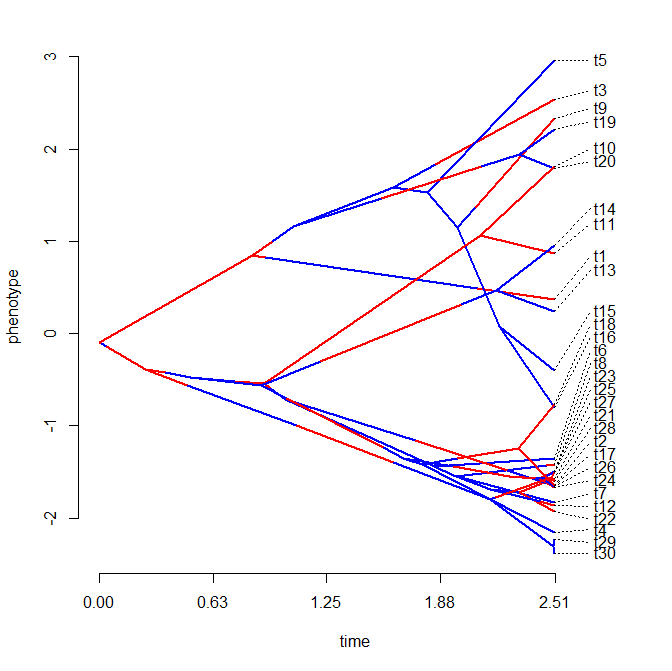
> cols<-setNames(c("blue","red"),letters[1:nrow(Q)])
> plotSimmap(mtrees[[1]],cols,pts=F,ftype="off")
Now let's compute the state frequencies from the stochastic maps for each internal node. These are our posterior probabilities for nodes:
> # function to compute the states
> foo<-function(x){
+ y<-sapply(x$maps,function(x) names(x)[1])
+ names(y)<-x$edge[,1]
+ y<-y[as.character(length(x$tip)+1:x$Nnode)]
+ return(y)
+ }
>
> AA<-sapply(mtrees,foo)
> piesA<-t(apply(AA,1,function(x,levels,Nsim) summary(factor(x,levels))/Nsim,levels=letters[1:3], Nsim=100))
> plot(tree,no.margin=TRUE,show.tip.label=F)
> nodelabels(pie=piesA,cex=0.6,piecol=cols)

Finally, let's compare to the generating map:
> # first compute the number of changes of each type
> XX<-countSimmap(mtrees,message=FALSE)
> colMeans(XX)
    N   a,a   a,b   b,a   b,b
28.65  0.00 10.88 17.77  0.00
> # compare to the true history
> countSimmap(tree,message=FALSE)
$N
[1] 27
$Tr
   a  b
a  0 11
b 16  0
> # now compute the mean overlap with the true history
> xx<-sapply(mtrees,map.overlap,tree)
> mean(xx)
[1] 0.9144295

I think that we can be pretty confident that make.simmap is doing what it's supposed to do; however please keep in mind that this version is brand new and has not been thoroughly tested. And, as Rich showed in pointing out this potential error to me, it is always wise to look behind the curtain - if possible - and don't hesitate to report any bugs, issues, or questionable results to me ASAP. I'll do whatever I can to address them.

Friday, March 15, 2013

Using plotBranchbyTrait to plot different style trees

A recent commenter pointed out something that I hadn't realized about the new phytools function, plotBranchbyTrait - that is, that it can be used to plot different styles of tree and that the branch coloring works (mostly) for all of them. This shouldn't have been a surprise - because, unlike most of my other tree plotting function, plotBranchbyTrait is really just a wrapper around ape's versatile plot.phylo function. Furthermore, I made a specific effort to migrate as much control of the operation of plot.phylo out to the phytools user. Nonetheless, it did not occur to me that plotBranchbyTrait(...,type="cladogram"), type="unrooted", or type="radial" would work or produce a nice looking result. In fact, they seem to work great - with one exception.... Here's a quick demo:

> tree<-pbtree(n=40)
> x<-fastBM(tree)
> plotBranchbyTrait(tree,x,mode="tips",type="cladogram", legend=F)
> plotBranchbyTrait(tree,x,mode="tips",type="unrooted", legend=F)

The only one that doesn't seem to work out quite right (as pointed out by Jonathan) is type="fan", where the 'horizontal' lines in the graph (actually, here circular lines) plot black:
> plotBranchbyTrait(tree,x,mode="tips",type="fan",legend=F)

New version of countSimmap for "multiPhylo" objects

I just posted a new version of countSimmap for an object of class "multiPhylo" that uses the method described in a recent post. Here's a quick demo:

> require(phytools)
> source("utilities.R")
> tree<-pbtree(n=100,scale=1)
> Q<-matrix(c(-2,1,1,1,-2,1,1,1,-2),3,3)
> colnames(Q)<-rownames(Q)<-LETTERS[1:nrow(Q)]
> tree<-sim.history(tree,Q)
> mtrees<-make.simmap(tree,tree$states,model="ER",nsim=10)
> XX<-countSimmap(mtrees)
> XX
$Tr
       N A,A A,B A,C B,A B,B B,C C,A C,B C,C
 [1,] 43   0  13  15   3   0   5   5   2   0
 [2,] 35   0  13  12   3   0   4   1   2   0
 [3,] 39   0  15  11   3   0   6   3   1   0
 [4,] 46   0  12  15   3   0   6   3   7   0
 [5,] 48   0   5   5  10   0  14   8   6   0
 [6,] 45   0  14  12   5   0   7   5   2   0
 [7,] 53   0  12  11  18   0   7   1   4   0
 [8,] 46   0   5   5   9   0   7  11   9   0
 [9,] 48   0  10   5   6   0  12   8   7   0
[10,] 49   0  16   8  15   0   6   3   1   0

$message
[1] "Column N is the total number of character changes on 
the tree"
[2] "Other columns give transitions x,y from x->y" 

That's it.

Wednesday, March 13, 2013

Applying countSimmap to a set of trees

I just received the following email request about the function countSimmap that counts the transitions on a mapped tree that's been created or read into memory:

I was wondering if this function (countSimmap) could work on SIMMAP files that contain multiple mappings (like the attached). I got it to work on single mappings like the example on the blog but get errors on my other files.

This is not too hard. Here's how we can do it using sapply:
library(phytools)
## first simulate a tree & some mapped histories
tree<-pbtree(n=100,1)
Q<-matrix(c(-2,1,1,1,-2,1,1,1,-2),3,3)
rownames(Q)<-colnames(Q)<-letters[1:3]
trees<-sim.history(tree,Q,nsim=10)

## now let's run the analysis using sapply
foo<-function(tree){
  XX<-countSimmap(tree)
  setNames(c(XX$N,as.vector(t(XX$Tr))),c("N",
    sapply(rownames(XX$Tr),paste,colnames(XX$Tr),sep=",")))
}
XX<-t(sapply(trees,foo))

And here are what the results look like for this toy example:
> XX
        N c,c c,a c,b a,c a,a a,b b,c b,a b,b
 [1,] 212   0  38  28  36   0  41  33  36   0
 [2,] 179   0  25  36  28   0  23  31  36   0
 [3,] 188   0  29  31  33   0  31  33  31   0
 [4,] 184   0  36  33  30   0  30  24  31   0
 [5,] 189   0  36  30  27   0  32  28  36   0
 [6,] 196   0  30  31  36   0  36  28  35   0
 [7,] 177   0  24  25  37   0  33  26  32   0
 [8,] 175   0  30  19  42   0  38  19  27   0
 [9,] 184   0  24  27  31   0  31  36  35   0
[10,] 214   0  41  47  36   0  30  32  28   0

That's it.

Small follow-up to rate-by-state method

This is a follow-up to my earlier post on attempting to measure the influence of the state of one continuous trait on the Brownian rate of a second.

First, the posted code had a small bug. Basically there is a superfluous internal loop that does nothing (except add to the run time). This got inserted while I was programming & testing the function, and I forgot to remove it. The updated version is here.

This new version of the function also has a method, logarithm=TRUE, which fits exp(ancestors of x)~contrasts(y). This just allows for the possibility that the rate changes as a multiplicative function of x, I think.

Finally, there is a new function - sim.ratebystate - which simulates under each of the assumed models. Here's a quick demo:

> tree<-pbtree(n=200,scale=1)
> source("ratebystate.R")
> XY<-sim.ratebystate(tree,sig2x=0.1,method="by.branch", plot=TRUE,beta=c(0,2))
> ratebystate(tree,XY[,"x"],XY[,"y"],method="by.branch")
$beta
[1] 2.069869
$r
[1] 0.2875908
$P
[1] 0.01
$corr
[1] "pearson"
$method
[1] "by.branch"

I also built a new version of phytools (phytools 0.2-26) that can be downloaded and installed from source.

New phytools version (phytools 0.2-25)

I just posted a new minor phytools release, phytools 0.2-25, that can be downloaded and installed from source.

> install.packages("phytools_0.2-25.tar.gz",type="source", repos=NULL)
* installing *source* package 'phytools' ...
** R
...
* DONE (phytools)

This package version contains a few new functions relative to the last minor phytools build (e.g., 1, 2), along with updates to some others including (most significantly) the phytools 'traitgram' function, phenogram.

Check it out - and please post any bugs or issues.

Tuesday, March 12, 2013

Investigating whether the rate of one continuous trait is influenced by the state of another (a somewhat ad hoc approach)

Yesterday, the following query was submitted to the R-SIG-phylo email listserve:

I have a continuous dependent variable (e.g. range size) and a few "independent" variables (e.g. body mass, encephalization ratio), and I want to test how the rate of evolution of the dependent variable is affected by the independent variables. The PCMs that I'm familiar with cannot be used to answer this question, because they usually try to predict the dependent variable based on the independent variables (e.g. PGLM) instead of looking at the rates of evolution.

Ideally, we'd take a model-based approach to this problem, as pointed out by Matt Pennell. Unfortunately, this has not yet been done. In its stead, however, it is not too difficult to devise a somewhat ad hoc, simulation-based alternative. Here was my proposal:

What about the admittedly ad hoc approach of computing the correlation between the states at ancestral nodes for x & the squared contrasts for corresponding nodes for y? Then you can generate a null distribution for the test statistic (say, a Pearson or Spearman rank correlation) by simulation. This seems to give reasonable type I error when the null is correct, and when I simulate under the alternative (i.e., the rate of Brownian evolution along a branch depends on the state at the originating node) it sometimes is significant.

Here is the function I proposed and submitted to the list to do this, I have since posted a more sophisticated method & function here.

ratebystate<-function(tree,x,y,nsim=100,method=c("pearson","spearman")){
   method<-method[1]
   if(!is.binary.tree(tree)) tree<-multi2di(tree)
   V<-phyl.vcv(cbind(x,y),vcv(tree),lambda=1)$R
   a<-fastAnc(tree,x)
   b<-pic(y,tree)[names(a)]^2
   r<-cor(a,b,method=method)
   beta<-setNames(lm(b~a)$coefficients[2],NULL)
   foo<-function(tree,V){
      XY<-sim.corrs(tree,V)
      a<-fastAnc(tree,XY[,1])
      b<-pic(XY[,2],tree)[names(a)]^2
      r<-cor(a,b,method=method)
      return(r)
   }
   r.null<-c(r,replicate(nsim-1,foo(tree,V)))
   P<-mean(abs(r.null)>=abs(r))
   return(list(beta=beta,r=r,P=P,method=method))
}

I was naturally somewhat curious about how it would do. To figure that out, we need to simulate under the null & alternative models. The null model is trivial, of course - constant-rate Brownian motion. The alternative model is a little trickier. Here, I see two different alternatives: (1) the rate of branches descended from each internal node is a linear function of the state at that node; or (2) the rate of each branch is a linear function of the average state along that edge, where we compute the average as the mean of the rootward and tipwards nodes subtending the edge. [**Note that in the simple function above, we explicitly assume (1); however in the full version I allow for either model to be assumed using method="by.node" for (1), and method="by.branch" for (2).]

Let's first simulate under the proposed alternative model and see if the result is reasonable. I will show option (2) here:

> require(phytools)
> # simulate tree
> tree<-pbtree(n=200,scale=1)
> # simulate continuous independent variable
> x<-fastBM(tree,internal=TRUE)
> # now *scale* the branch lengths of the tree
> # by the mean of x for each edge
> ss<-rowMeans(matrix(x[tree$edge],nrow(tree$edge),2))
> zz<-tree; zz$edge.length<-zz$edge.length*(ss-min(ss))
> # visualize the scaled tree by trait relationship
> phenogram(zz,x,type="b",color="blue",ftype="off", xlab="expected variance",ylab="independent variable (x)")
> # now simulate y
> y<-fastBM(zz)
> # now let's fit our model
> source("ratebystate.R")
> ratebystate(tree,x[tree$tip.label],y,method="by.branch")
$beta
[1] 1.169129
$r
[1] 0.3187849
$P
[1] 0.01
$corr
[1] "pearson"
$method
[1] "by.branch"

Well, one simulation test does not a new method make. Here's some code that I used to run simulations under the null & alternative models [actually here under model (1), from above]:
# simulate under the null
f.null<-function(){
  tree<-pbtree(n=100)
  x<-fastBM(tree)
  y<-fastBM(tree)
  ratebystate(tree,x,y,message=FALSE)
}
sim.null<-t(replicate(400,f.null()))

# simulate under the alternative (model 1)
f.alt<-function(){
  tree<-pbtree(n=100)
  x<-fastBM(tree,internal=TRUE)
  nodes<-x[1:tree$Nnode+length(tree$tip.label)]
  zz<-tree; zz$edge.length<-zz$edge.length*(nodes[as.character(tree$edge[,1])]-min(nodes))
  y<-fastBM(zz)
  ratebystate(tree,x[tree$tip.label],y,message=FALSE)
}
sim.alt<-t(replicate(400,f.alt()))

And here are the results:
> colMeans(sim.null)
      beta           r           P
0.006199303 0.004057295 0.516675000
> mean(sim.null[,"P"]<0.05)
[1] 0.03
> colMeans(sim.alt)
    beta         r         P
1.0114919 0.2617357 0.0742000
> mean(sim.alt[,"P"]<0.05)
[1] 0.6775

So it would seem (based on these very limited simulations) that the method has type I error near or below the nominal level. Furthermore, the power is not too bad when the alternative hypothesis is correct. Finally - the mean slope of the regression between contrasts variance and ancestral states is actually very close to our generating relationship - in this case 1.0.

That's it.

Monday, March 11, 2013

Neat new function to color branches by trait value

I had a user request yesterday for a function that would plot edge colors by probability - for example, if we have a value on [0, 1] for each edge in the tree - how do we use a built-in color palette in R to plot the tree using these edges as our colors? I think that the idea is somewhat akin to what contMap or densityMap accomplish; however if all we want is to plot each edge a different color, the 'ape' function plot.phylo is just fine at doing that.

I wrote a new function, plotBranchbyTrait, which automates this - calling plot.phylo internally; but the central piece of code used by the function is relatively simple. It merely takes our probabilities or reconstructed trait values along branches of the tree and translates them to colors from a palette as follows (using, in this case, a blue→red color map):
cols<-rainbow(1000,start=0.7,end=0) # blue->red
if(is.null(xlims)) xlims<-range(x)+c(-tol,tol)
breaks<-0:1000/1000*(xlims[2]-xlims[1])+xlims[1]
whichColor<-function(p,cols,breaks){
  i<-1
  while(p>=breaks[i]&&p>breaks[i+1]) i<-i+1
  cols[i]
}
colors<-sapply(x,whichColor,cols=cols,breaks=breaks)

What we come out with is a vector of colors to use as input in the argument plot.phylo.

I also have another internally called function, add.color.map, which takes user input for location and then plots a translation map (that also serves as a scale bar, as in, for instance, densityMap). I'd never done this before, but getting an interactively user supplied position for the color map was pretty easy. Here is the code snippet that I used:
cat("Click where you want to draw the bar\n")
x<-unlist(locator(1))
y<-x[2]
x<-x[1]

This is based on something similar in the ape function add.scale.bar.

One warning to the user - the function hangs before printing the "Click where you want to draw the bar" and waits for you to supply the location before the prompt! Not sure how to fix this.

The function has three different modes. mode="edges" uses the user supplied trait value for all the edges in the tree. The input values should be in the row order of tree$edge. mode="tips" just takes tip values and it reconstructs ancestral states by using fastAnc to compute the ancestral node states, and the averages the tipward and rootward states for each edge to get the plotted color. mode="nodes" does the same averaging, but the tip and node values are user supplied.

Here's a quick and dirty demo:
> source("plotBranchbyTrait.R") # load source
> # simplest use: ancestral BM values
> tree<-pbtree(n=40)
> x<-fastBM(tree)
> plotBranchbyTrait(tree,x,method="tips")
Click where you want to draw the bar
> # now let's say we have probabilities for each edge
> pp<-fastBM(tree,bounds=c(0,1),internal=TRUE)
> p<-rowMeans(matrix(pp[tree$edge],nrow(tree$edge),2))
> plotBranchbyTrait(tree,p,xlims=c(0,1),palette="gray")
Click where you want to draw the bar

Other methods in this function should be fairly self explanatory, I hope.

That's it.

Saturday, March 9, 2013

Significant update to phenogram

The phytools function phenogram does a projection of the phylogeny into a space defined by time since the root (on the x axis) and phenotype (on y). It has some nice features, for instance it can map the state of a discrete character on the tree, but it also had a couple of small bugs associated with labeling the leaves - specifically, the alignment of tip labels is messed up, and it sometimes did not leave enough whitespace right of the tips for labels to be printed.

I decided to do a significant overhaul of phenogram to both try and fix these issues as well as to enable a lot more user control of plotting within the function.

Fixing the text alignment was a piece of cake; however allocating enough whitespace for plotting tip labels turned out to be a much more complicated issue. This is not something that I've really dealt with in tree plotting before because in my other major tree plotting function, plotSimmap, the function circumvents the issue by fixing the plotting area to a unit in length, and then fractioning that area into a part for the tree and a second part for tip labels. (This works really well, but introduces complications when you want to include a legend - e.g., here.)

Let me try to explain why this (probably) seemingly trivial issue can be such a pain in the butt. Now, we have a function strwidth which will give us the width (in various units) of a plotted string. The difficulty arises if we want to tie the limits of a plotting area to a call of strwidth. This is because strwidth(...,units="user") (the default) will only work properly after our plotting device has been opened. This means that it can't be used to specify the dimensions of the plotting area - paradoxical if the point of specifying a specific set of dimensions for plotting is specifically to leave space for plotted strings! The solution* turns out to be first pull the horizontal dimension in inches of our plotting device out using par("pin"); then finding the maximum width of our tip labels (again, in inches) on the plotting devices; and then, finally, using numerical optimization to find the ratio of our units (time since the root, in this case) and inches that allows us to use the whole plotting devices when the tip labels are also plotted. The way this looks in practice is as follows:
# node heights
H<-nodeHeights(tree)
# width of the plotting device, in inches
pp<-par("pin")[1]
# string width on the plotting device, in inches
# (includes label offset)
sw<-fsize*(max(strwidth(tree$tip.label,units="inches")))+   offset*fsize*max(strwidth(tree$tip.label,
  units="inches"))/max(nchar(tree$tip.label))
# find the ratio of inches:units that fills the
# plotting window
alp<-optimize(function(a,H,sw,pp)
  (a*1.04*max(H)+sw-pp)^2,
  H=H,sw=sw,pp=pp,interval=c(0,1e6))$minimum
# set x-limits
xlim<-c(min(H),max(H)+sw/alp)

(*This solution is derived from something that Emmanuel Paradis did in the ape function plot.phylo. Thanks Emmanuel!)

While I was at it, I decided to migrate a lot of other controls over plotting to the user. This will be in the function documentation for the next phytools version, but here's a quick demo:
> source("phenogram.R")
> tree<-pbtree(n=20)
> x<-exp(fastBM(tree))
> phenogram(tree,x,log="y",colors="blue",type="b", offset=0.5,xlab="millions of years",ylab="body size", main="Body Size Evolution")

The source code for the new version of phenogram is here. It will also be updated in the next version of phytools.