Phylomorphospace plotting

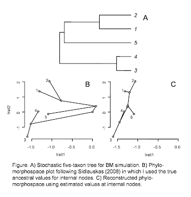
I created panels (B) and (C) of the plot at right using a new function I wrote to reproduce the so-called "phylo-morphospace" graphing method of Sidlauskas (2008). Note that this function is available without guarantees, but I would happy to hear about its success or failure on your dataset.

The function, which is available here, takes a tree and two matrices as input. The first matrix is n x 2 and contains the tip values for two traits in n species on the tree (n=5 in this case). The second matrixis m x 2 for m internal nodes and contains the values (known or estimated) for each internal node in the tree, including the root.

To create the panels, I first simulated BM evolution for two traits on the five-taxon stochastic tree in panel (A). I stored both the ancestral trait values and the tip values for terminal species (more on that later).

For panel (B) I sent my function the tip values, along with the known values for internal nodes from the simulation. For panel (C), I first estimated internal node states for the two characters using the "ape" function ace() (ancestral character estimation) under ML. This latter scenario would be more typical of empirical studies.

The contrast between (B) and (C) is pretty neat in this case. This is because in the simulation the true states at internal nodes are nearly invariably (with the exception of the MRCA of species 3 & 4) beyond the range of the observed data for the terminal species in our tree.

I will write more on programming the phylomorphospace plotting function as well as on simulating data while retaining the states at internal nodes in subsequent posts.

Reading SIMMAP format trees, part II

In my last post I described a new function (presently available from my beta version R phylogenetics page) to read SIMMAP v1.0 format trees into R. Trees in this format have roughly the following form:
((A:{0,0.3:1,0.4:0,0.3},B:{0,1.0}):{0,1.0},(C:{0,0.25:1,0.75},D:{0,1.0}):{0,1.0});
The tree above would correspond to the visual mapping of the figure, right, in which blue branches represent state "0" and red branches state "1."
The most obvious way to code a function to read the tree above into R would be to take Paradis's "ape" function read.tree() and modify it to take the { parenthetical } form of branch lengths. However, the most obvious solution is not always the easiest. What I quickly realized was that it would be much easier to first parse the tree into two (or more) Newick format trees for each state of the binary character. All trees in this case would have the same topology, but their branch lengths would correspond to the time spent in each state on that tree. For instance from the tree above, we would obtain the Newick trees as follows:
"0" : ((A:0.6,B:1.0):1.0,(C:0.25,D:1.0):1.0); and
"1" : ((A:0.4,B:0.0):0.0,(C:0.75,D:0.0):0.0);.
Note that doing this destroys all information about the order of states along edges. This information is unimportant for some analyses (such as O'Meara et al. 2006), but might be critical for others.
We now simply call read.tree() on each of the state trees above to create a "multiPhylo" object which contains a list of the trees for each mapped state. To create our SIMMAP tree in memory, then, we first copy the topology of any of the state trees in our list into our mapped tree (remember, they all have the same topology), and then we create a matrix mapped.edge with the time on each edge (rows) from each state tree (columns). These are just the $edge.length branch length vectors from each tree. We then add across columns of mapped.edge to get the total length of each edge.
The product here is an object of class "phylo" but with the additional element, our matrix from earlier $mapped.edge, which contains the times spent in each state on each edge of the tree. And we're done!
I should note that in creating this function I did in fact borrow and modify a chunk of code from the "ape" function read.nexus(). This allowed me to read not only Phylip style tree files, as given above, but also the more complicated Nexus style output files created by SIMMAP.

Reading SIMMAP trees into R

Stochastic character mapping, originally due to Nielsen (2001, 2002) and Huelsenbeck et al. (2003) is a procedure whereby mutations or character substitutions are mapped onto the nodes and branches of a phylogenetic tree. Maps are generated stochastically, but with probability equal to their posterior probability given our transition model. Sampling stochastic character maps, then, may be a good way to capture information about both the states at internal positions in the tree, as well as the timing of character substitution through the phylogeny. As noted in an earlier post, the background of this blog are visualized stochastic character maps for "ecomorph" mapped on the Caribbean Anolis tree (from Mahler et al. 2010).

The program SIMMAP for stochastic mutational mapping was developed by Jonathan Bollback. It performs stochastic mutation mapping, and outputs stochastically mapped trees to file using a modified Newick format. Since stochastic character maps can be very useful for certain kinds of downstream phylogenetic analysis, I was very interested in writing a function that would read these modified Newick trees into R.

The basic format of stochastic character mapped phylogenies in v1.0 of SIMMAP is as follows:

((A:{0,0.3:1,0.4:0,0.3},B:{0,1.0}):{0,1.0},(C:{0,0.25:1,0.75},D:{0,1.0}):{0,1.0});

This is comparable to the standard Newick style tree except that branch lengths have been replaced by { curly brackets } according to the following convention: { state i, time spent in state i : state j, time spent in state j : etc. }.

I'm happy to announce that I have now developed usable code to read SIMMAP v1.0 trees in R. This function, read.simmap(), accepts either or Phylip or Nexus style input files (the latter courtesy in large part to code borrowed from the "ape" function read.tree()). My function creates a modified "phylo" object, with the additional element $mapped.edge which is a matrix containing the time spent in each state (columns) on each edge (rows) of the tree. The source code for this function is available as a beta test version from my R phylogenetics page, here, along with some very basic description of use.

Unfortunately, this announcement comes with a hitch. In the most recent release of SIMMAP (v1.5) Bollback has updated the SIMMAP tree format so that the tree above would be represented as follows:

((A:[&map={0,0.3,1,0.4,0,0.3}]1.0,B:[&map={0}]1.0):[&map={0}]1.0,(C:[&map={0,0.25,1,0.75}]1.0,D:[&map={0}]1.0):[&map={0}]1.0);

The reason for this, I surmise, is that now these trees conform to the Newick standard (in which, by convention, text inside [ hard brackets ] is ignored) and thus can be read by programs not specifically designed to read SIMMAP style trees. Unfortunately, Bollback does not provide any means of converting between old and new formatted trees.

I'm working on reading the new SIMMAP format into R as an option in my read.simmap() function. I will keep readers of this blog up to date on my progress on this problem. I will also work on adding the capacity to retain the order of states on each edge, as the present version of my function destroys this information during read-in (retaining only the total time spent in each state on each edge).

Please feel free to test my function with SIMMAP v1.o formatted trees and let me know what you find.

R-phylogenetics beta distribution

The focus of this blog is, as noted earlier, to chronicle method development. As I do this, I will also post beta test versions of a lot of my R code on my R-phylogenetics test version page. (Note that although I will keep this link current, the actual URL may change as I migrate my research pages to University of Massachusetts Boston, where I will be starting in the biology department next month.)

**As of Feb. 2, 2012 I have finally started to migrate my code to a new phytools development page here. I am making every attempt to update all the links of this blog & I will keep the old URL active for as long as possible.

Explanation of the background

The background to this blog is (many iterations of) a phylogenetic tree for 100 species of Caribbean Anolis lizards; specifically the phylogeny of Mahler et al. (2010). The colors mapped on the tree represent one stochastic character map of the famous Anolis ecomorphs. Note that not all Caribbean Anolis in this phylogeny belong to an ecomorph; these non-ecomorph species are plotted with dark orange branches. The circular tree was created with the wonderful program FigTree v1.3.1 (Rambaut 2009). The stochastic mapping was generated using the program SIMMAP v1.0 (Bollback et al. 2006).

Future home of phytools

This website will be the future home of a web-log dedicated to the development and use of phylogenetic tools for comparative biology.