Improvements/bug-fixes in plotBranchbyTrait

Unlike most of the phylogeny plotting functions of phytools which use the multifunctional plotting function plotSimmap internally, the phytools function plotBranchbyTrait is nothing more than a fancy wrapper for the ape S3 plotting method plot.phylo.

The other day a phytools user reported a couple of bugs: (1) when type="fan" the labels plot horizontally instead of radially, as you might expect; and (2) also type="fan" the scale of the plot is all messed up if legend=TRUE and prompt=FALSE (conveniently, the default).

All this havoc resulted just by providing default options for some of things that were well designed to work with certain plot types, but poorly designed for others. I have just posted a fixed version of this function; however users interested in this update should probably just install the latest phytools version from source.

Here is a quick demo:

> require(phytools)
> packageVersion("phytools")
[1] ‘0.4.27’
> tree<-pbtree(n=50,scale=1)
> x<-fastBM(tree)
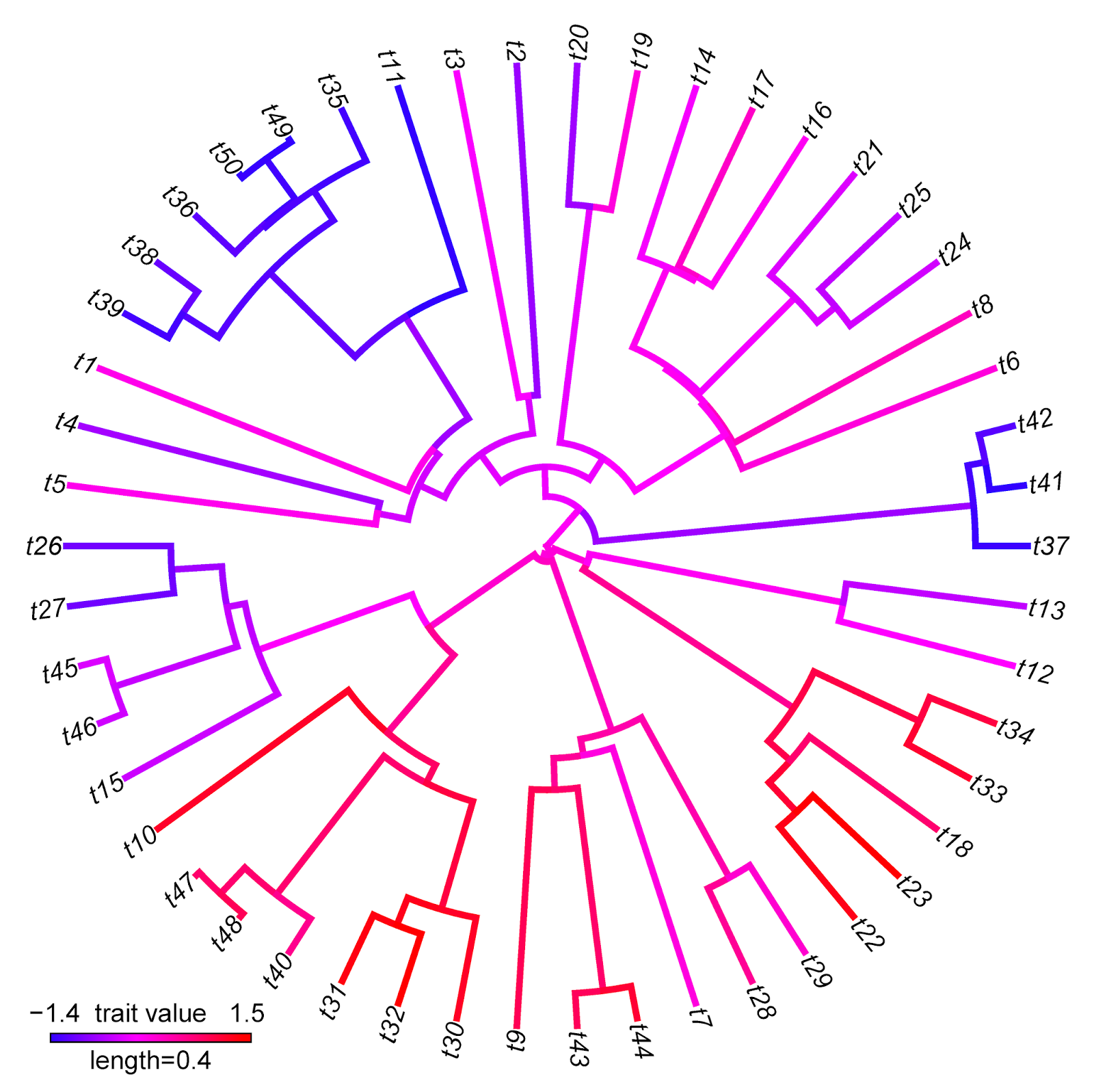
> plotBranchbyTrait(tree,x,mode="tips",type="fan", legend=0.4)

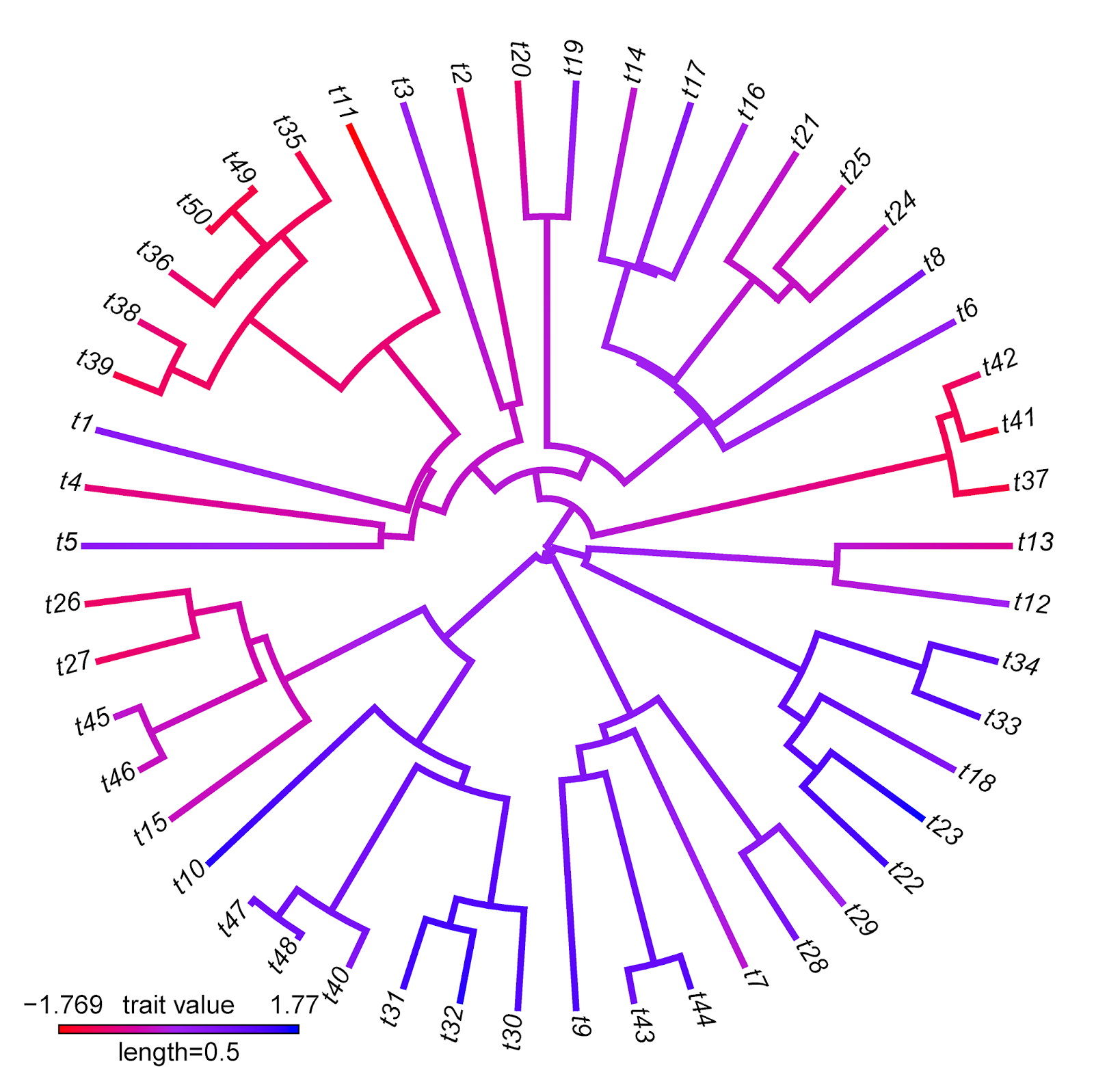
Note that for this specific type of visualization, I would strongly recommend trying my function contMap. Here's a demo of how that would work:

> obj<-contMap(tree,x,plot=FALSE)
> obj<-setMap(obj,colors=c("red","purple","blue"), space="Lab")
> plot(obj,type="fan",outline=FALSE)

plotBranchbyTrait makes more sense, of course, when we have a trait value associated with each edge that we want to plot on the tree without any interpolation.

Note that there are some interesting differences between these two visualizations that reflect differences between the methods implemented. For instance, the range of trait values in plotBranchbyTrait(...,mode="tips") is narrower than for contMap. This is because plotBranchbyTrait(...,mode="tips"), to get the plotted values for each edge, takes the known or estimated trait values at each end of the edge and averages them. This will invariably contract the range of plotted values when compared to the true range.

Bug fix for S3 plotting method for objects of class "describe.simmap"

In recent phytools versions the phytools function describe.simmap returns an object of class "describe.simmap" which, if plotted, shows a phylogeny with posterior probabilities from stochastic mapping shown as pie charts at each node and tip of the tree. Unfortunately, when I switched the internal tree plotting function from ape's plot.phylo to plotTree in phytools, I made a mistake in setting the automatic offset of tip labels such that labels are frequently plotted outside the plotting window. This bug was reported to me today by a colleague and I just posted a new version of phytools with the bug in this plotting method fixed. This phytools version (>=0.4-26) can be downloaded from the phytools page and installed from source. Obviously, this fix will also be in subsequent CRAN releases of the phytools package.

Update to locate.yeti permitting the missing tip to attach below the root node

I just updated the phytools function locate.yeti (a method to attach a missing tip to an ultrametric base tree using continuous character data) so that the missing leaf is now permitted to attach below the root node.

When I first started working on this, I initially mistakenly thought that I would have to add one additional parameter to when attaching a new leaf to the root node - that being the length of the edge leading to the tip. Actually, this is not the case. Whereas for a leaf attached to an edge we have to optimize the position along the edge from whence the lineage splits; in the case of a leaf attached to the root we only have to optimize its total length. Since our tree is invariably ultrametric - the lengths of the root stem and the terminal edge can be found by simply midpoint rooting our phylogeny.

The new version of locate.yeti is here; however since locate.yeti uses phytools internal functions it is probably best & easiest to simply install the latest non-CRAN phytools version.

Here's a quick demo using a phylogeny in which the true position of the missing lineage is sister to our ultrametric base tree:

> packageVersion("phytools")
[1] ‘0.4.25’
> tree<-pbtree(n=26,tip.label=LETTERS,scale=1)
> tt<-bind.tip(tree,where=length(tree$tip.label)+1,
edge.length=1.2*max(nodeHeights(tree)),
tip="Missing-lineage")
> tt<-midpoint.root(tt)
> ## this is the full true tree
> plotTree(tt)

> ## simulate on the full tree
> X<-fastBM(tt,nsim=10)
> ## place our missing taxon
> mltree<-locate.yeti(tree,X,method="exhaustive")
Optimizing the phylogenetic position of Missing-lineage. Please wait....
Done.
> mltree$logL
[1] -221.0057
> plotTree(mltree)

Although it's pretty obvious that we have the correct tree in this case, we can also quantify it:

> require(phangorn)
Loading required package: phangorn
> RF.dist(tt,mltree)
[1] 0
> require(Rphylip)
Loading required package: Rphylip
> Rtreedist(tt,trees2=mltree,quiet=TRUE)
          2,1
1,1 0.0862447

That's pretty much it for now.

New user controls in phylo.to.map

I just posted a version of the phytools function phylo.to.map, which can be used to project a tree onto a geographic map. Based on some user feedback, including at the Latin American Macroevolutionary Workshop we just held at the Universidad de los Andes in Bogotá, Colombia, I have added a couple of new features & attributes to the function.

First, the function now automatically removes the underscore character ("_") from within species names. Note that this is only for type="phylogram", not type="direct"; although in the latter case it can easily be done manually.

Second, again for type="phylogram", the lines connecting the tree to locations on a geographic map now (by default) arise from the end of the tip label - rather than from the tip itself.

Finally, third, the function now allows user control of the color of both the dashed lines & points connecting species labels to their geographic locations (for type="phylogram"); and of the both the lines and tip dot colors (for type="direct".

These updates are in the latest non-CRAN phytools build. Here's a quick demo:

> packageVersion("phytools") [1] ‘0.4.24’
> ## simulate some realistic looking data
> foo<-function() paste(c(sample(LETTERS,1),
sample(letters,round(runif(n=1,min=3,max=5))),"_",
sample(letters,round(runif(n=1,min=4,max=6)))),
collapse="")
> tree<-pbtree(n=40,tip.label=replicate(40,foo()))
> tree$edge.length<-tree$edge.length*
100/max(nodeHeights(tree))
> lat<-fastBM(tree,sig2=10,bounds=c(-90,90))
> long<-fastBM(tree,sig2=20,bounds=c(-180,180))
> X<-cbind(lat,long)
> ## ok, first the (new) standard plot:
> obj<-phylo.to.map(tree,X,ftype="i",fsize=0.7,
asp=1.2,split=c(0.5,0.5))
objective: 302
...
objective: 220
objective: 218
objective: 218

> ## now let's change the colors:
> plot(obj,colors=c("blue","red"),ftype="i",fsize=0.7,
asp=1.2,split=c(0.5,0.5))

> ## direct projection with different colors
> plot(obj,type="direct",colors=c("red","black"),
fsize=0.7)

That's it.

Principal components rotation of ancestral states; or ancestral state reconstruction of PC scores?

I recently fielded the following query:

From what I understand, the phylomorphospace function allows the mapping of the phylogeny on a morphospace defined by 2 characters/traits. However, I'm using multivariate data from a morphometric analysis, and the shape variation is explained by a lot of axes. The first 2 PCs can approximate the shape variation, but my question is: how do you calculate ancestral nodes using all the PC scores, or all of your fourier coefficients if using this method? Is it possible? Do you calculate the nodes on the PCs you are interested in? Or do you calculate the nodes on all your variables and then project them in the desired shape space?

So, in essence, should we perform ancestral state reconstruction on our original characters and then rotate them using the PC loadings; or should we first run phylogenetic PCA and then perform ancestral state reconstruction on the PC scores for species?

Well, the answer is - it doesn't matter. We will obtain the same ancestral state reconstructions for our PCs regardless of our order of operations. This could no doubt be proved analytically, but it is also straightforward to demonstrate via simulation as follows.

First, simulate tree & data:

> ## stochastic pure-birth tree
> tree<-pbtree(n=26,tip.label=LETTERS)
> ## random covariance matrix
> L<-matrix(rnorm(16),4)
> L[upper.tri(L)]<-0
> V<-L%*%t(L)
> ## simulated correlated character evolution on the tree
> X<-sim.corrs(tree,vcv=V)

Now, we can do our two analyses - first compute ancestral states on the original data & rotate using the phylogenetic PCA loadings; and then rotate our tip data, and reconstruct ancestral states for the PC scores:

> ## perform phylogenetic PCA
> pca<-phyl.pca(tree,X)
> ## reconstruct ancestral states for original data
> A<-apply(X,2,fastAnc,tree=tree)
> ## rotate in PC space
> ## compute phylogenetic means for calculation
> M<-matrix(rep(A[1,],nrow(A)),nrow(A),ncol(A),byrow=TRUE)
> rotatedA<-(A-M)%*%pca$Evec
> ## now compute ancestral states for PCA scores
> S<-apply(pca$S,2,fastAnc,tree=tree)

Now we can compare them:

> plot(rotatedA,S)

That's it.

New version of read.newick that can read root node labels

The phytools function read.newick is a slower, but slightly more robust Newick tree reader than read.tree in the ape package - specifically in that it permits certain types of 'badly conformed' Newick strings, such as those containing singleton nodes.

It's Achilles heel, however, has been that it does not permit a node label for the root node of the tree. The fix for this was simple and was supplied to me by Joseph Brown. The updated function code is here & also in the latest non-CRAN phytools version (phytools >= 0.4-23) here.

Bug fix in make.simmap for multi-state data and non-reversible model of evolution

In response to an R-sig-phylo query about stochastic mapping in phytools I wrote:

I can answer the three questions that pertain to phytools:

(1) The function make.simmap has a bug for non-reversible models when the input character has more than 2 states. This has to do with the algorithm for simulating changes along edges where the correct waiting time is simulated, but then the states at the end of the waiting time are chosen with the incorrect probabilities. This will sometimes cause make.simmap to hang for a long time. This does not affect the states simulated at nodes (which occurs first) and should not affect stochastic character mapping at all for binary characters or any reversible model of character evolution. I have posted a fixed version here - but you can also install a version of phytools containing this update here. Use phytools >= 0.4-22.

(2) You should look into the function describe.simmap to summarize the time spent in each state, etc., from stochastic character mapping using make.simmap..

(3) To simulate stochastic character histories you can use the phytools function sim.history. Note, though, that the matrix Q is the transpose of the fitted value of Q from make.simmap. Sorry about this. That means to simulate stochastic character histories on your tree you can do:

## stochastic mapping:
mtrees<-make.simmap(tree,x,model="ARD",nsim=100)
## summarize results
obj<-describe.simmap(mtrees)
obj
plot(obj) ## PP at nodes from stochastic mapping
fitted.Q<-mtrees[[1]]$Q
## simulate under fitted model
simhistories<-sim.history(tree,t(fitted.Q),nsim=100,anc=rstate(obj$ace[1,]))

The last part (anc=rstate(obj$ace[1,])) is necessary if you have non-reversibility, because this way you are picking from the posterior distribution at the root from your real data.

In addition, sim.history does not permit any columns (rows in the matrix from make.simmap) to be equal to 0.0 (which we will have if we have a truly non-reversible character). To resolve this, you can do something like:

ii<-which(diag(fitted.Q)==0)
fitted.Q[ii,-ii]<-max(nodeHeights(tree))*1e-12
fitted.Q[ii,ii]<--sum(fitted.Q[ii,])
simhistories<-sim.history(tree,t(fitted.Q),nsim=100,anc=rstate(obj$ace[1,]))