Updates to plot.phylo.to.map and application to phylogeographic dataset

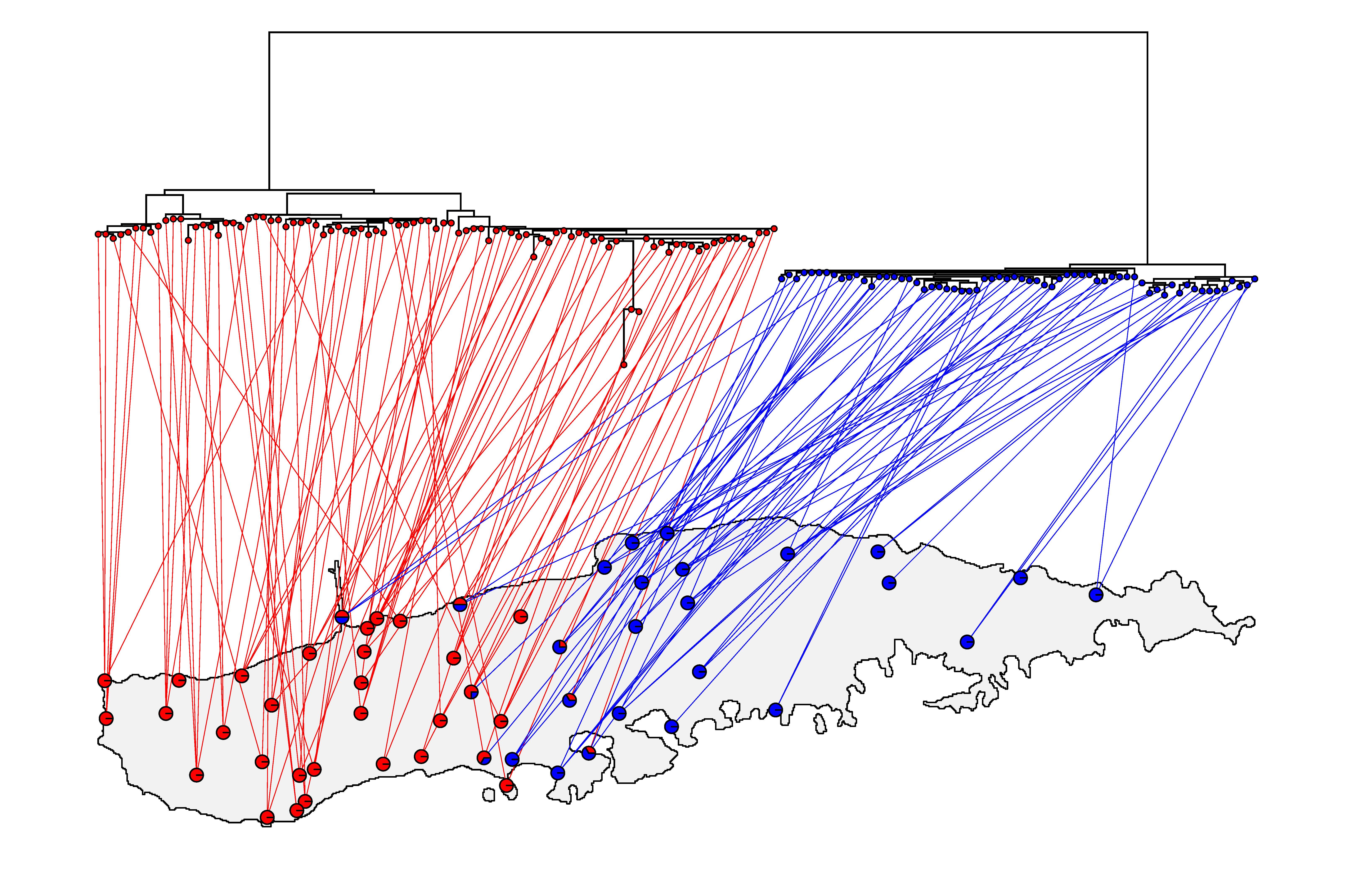
I just posted an update to plot.phylo.to.map that allows user control of the colors of both the plotted points and the linking lines. To obtain this update, install phytools from GitHub (using, for instance, devtools).

The following demonstrates the application of this updated version to some phylogeographic data from Isla Vieques in the Puerto Rican Bank archipelago.

## load libraries
library(phytools)
library(phangorn)
library(plotrix)
library(mapdata)

## read files
tree<-read.nexus("IPS_RAxMLtree_GTRGI.txt") ## tree
X<-read.csv("08.14 Vieques all data.csv",
    header=TRUE) ## data, incl. coordinates
PR<-read.csv("PR MAP Coordinates.csv",
    row.names=1) ## higher res PR map

## pull out sample names
ss<-as.character(X$Series)
tips<-vector()

## they match imperfectly, so let's search for each one
## and rename the tip labels in our tree
for(i in 1:length(ss)){
    ii<-grep(ss[i],tree$tip.label)
    if(length(ii)>0){
        tree$tip.label[ii]<-ss[i]
        tips<-c(tips,ss[i])
    }
}
## dropping tips not in our sample
tree<-drop.tip(tree,setdiff(tree$tip.label,tips))

## get coordinates, dropping points not in our tree
ii<-sapply(tips,function(x,y) which(y==x),y=ss)
coords<-cbind(X$Lat[ii],X$Long[ii])
rownames(coords)<-tips
colnames(coords)<-c("lat","long")

## now let's deal with our high res map as it needs curation
## isolate the island of Vieques
ii<-which(PR[,1]>(-65.7))
jj<-which(PR[,1]<(-65.2))
ij<-intersect(ii,jj)
kk<-which(PR[,2]>18.05)
ll<-which(PR[,2]<18.17)
kl<-intersect(kk,ll)
ind<-intersect(ij,kl)
## check
plot(PR[ind,],asp=1,pch=19,cex=0.7)

x<-PR[ind,1]
y<-PR[ind,2]

## there are some offshore islands, so I need to further
## curate the coordinates so that these are plotted as separate
x<-c(x[1:20],NA,x[21:54],NA,x[55:length(x)])
y<-c(y[1:20],NA,y[21:54],NA,y[55:length(y)])

## now create our "phylo.to.map" object, but without plotting
obj<-phylo.to.map(tree,coords,
    database="worldHires",regions="Puerto Rico",
    plot=FALSE)

## objective: 5598

## objective: 4080
## objective: 4080

## objective: 4078

## objective: 4070
## objective: 4070

## objective: 4064

## objective: 4060

## objective: 4058
## objective: 4058
## objective: 4058
## objective: 4058
## objective: 4058

## objective: 4056
## objective: 4056
## objective: 4056
## objective: 4056
## objective: 4056
## objective: 4056
## objective: 4056
## objective: 4056

## objective: 2958

## objective: 2934
## objective: 2934
## objective: 2934
## objective: 2934

## objective: 2908
## objective: 2908
## objective: 2908

## objective: 2906
## objective: 2906

## objective: 2904
## objective: 2904

## objective: 2888
## objective: 2888
## objective: 2888

## objective: 2878

## objective: 2868
## objective: 2868

## objective: 2864
## objective: 2864
## objective: 2864

## objective: 2858
## objective: 2858
## objective: 2858

## objective: 2856

## objective: 2854
## objective: 2854
## objective: 2854
## objective: 2854
## objective: 2854
## objective: 2854

## objective: 2852
## objective: 2852
## objective: 2852
## objective: 2852
## objective: 2852
## objective: 2852
## objective: 2852
## objective: 2852

## objective: 2848
## objective: 2848
## objective: 2848
## objective: 2848
## objective: 2848
## objective: 2848

## objective: 2826

## objective: 2812

## objective: 2790
## objective: 2790
## objective: 2790

## objective: 2772
## objective: 2772
## objective: 2772
## objective: 2772
## objective: 2772

## objective: 2770
## objective: 2770

## objective: 2768

## objective: 2766

## objective: 2746
## objective: 2746
## objective: 2746

## objective: 2744
## objective: 2744
## objective: 2744
## objective: 2744
## objective: 2744
## objective: 2744
## objective: 2744
## objective: 2744

## objective: 2132
## objective: 2132
## objective: 2132
## objective: 2132
## objective: 2132

## objective: 2088
## objective: 2088

## objective: 2036
## objective: 2036
## objective: 2036

## objective: 2030

## objective: 2028

## objective: 2026
## objective: 2026

## objective: 1996
## objective: 1996

## objective: 1978
## objective: 1978
## objective: 1978
## objective: 1978
## objective: 1978
## objective: 1978
## objective: 1978

## objective: 1958
## objective: 1958

## objective: 1956
## objective: 1956
## objective: 1956

## objective: 1898

## objective: 1870

## objective: 1866
## objective: 1866

## objective: 1864

## objective: 1860
## objective: 1860
## objective: 1860
## objective: 1860
## objective: 1860
## objective: 1860
## objective: 1860
## objective: 1860
## objective: 1860
## objective: 1860
## objective: 1860
## objective: 1860
## objective: 1860
## objective: 1860

## objective: 1858
## objective: 1858
## objective: 1858
## objective: 1858
## objective: 1858
## objective: 1858
## objective: 1858
## objective: 1858

## objective: 1856
## objective: 1856

## objective: 1854
## objective: 1854

## objective: 1852

## objective: 1850

## objective: 1848

## objective: 1846

## substitute our higher resolution map
obj$map$x<-x
obj$map$y<-y
obj$map$range<-c(range(PR[ind,1]),range(PR[ind,2]))

## now I want to color different clade members different
## colors. The two clades split at the root, so this is
## easy
tmp<-tree$edge[which(tree$edge[,1]==(Ntip(tree)+1)),2]
left<-tmp[2]
right<-tmp[1]
red<-tree$tip.label[Descendants(tree,left,"tips")[[1]]]
blue<-tree$tip.label[Descendants(tree,right,"tips")[[1]]]

## create a color matrix for points and links
colors<-matrix(NA,nrow(coords),2,dimnames=list(rownames(coords)))
for(i in 1:length(red))
    colors[red[i],1:2]<-c("red","red")
for(i in 1:length(blue))
    colors[blue[i],1:2]<-c("blue","blue")

## now we can plot our object
plot(obj,ftype="off",lwd=c(1.25,0.5),ylim=c(18.07,18.2),
    colors=colors,lty="solid")

## finally, I want to overlay clade membership frequency by
## site
sites<-unique(coords[,1]) ## assume each site has a unique latitude
for(i in 1:length(sites)){
    nred<-sum(coords[red,]==sites[i])
    nblue<-sum(coords[blue,]==sites[i])
    x<-c(nred,nblue)/sum(nred+nblue)
    floating.pie(coords[which(coords[,1]==sites[i])[1],2],
        sites[i],x,edges=200,radius=0.0018,col=c("red","blue")[x>0])
}

This can also be saved as a much nicer looking PDF (or click on image above).

That's all.