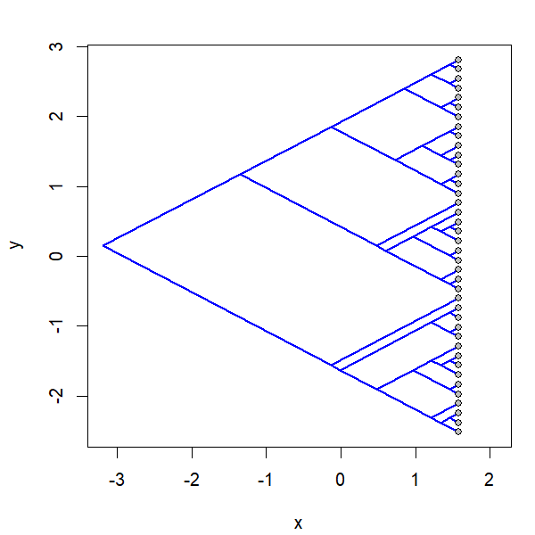
Yesterday I posted a function to animation the projection of a phylogeny into so-called 'phylomorphospace.' Basically the function morphs a cladogram into morphospace.
I have now updated this function & added it to the phytools package so it can be obtained merly by updating phytools from GitHub using devtools
The update consisted of doing a few things:
1) I eliminated a (hard to notice except when converted to .gif) first blank
plotting device using par(new=TRUE).
2) I allow users to morph backwards from phylomorphospace to tree, forwards, or both.
Complete code of the function can be seen above; however for the plot
below I also made a small 'fix' (using fix) the internally
used phylomorphospace which I intend to add as an option
later.
Here's a demo:
library(phytools)
packageVersion("phytools")
## [1] '0.6.58'
tree
##
## Phylogenetic tree with 40 tips and 39 internal nodes.
##
## Tip labels:
##  t19, t20, t5, t15, t16, t8, ...
##
## Rooted; includes branch lengths.
X
##            [,1]       [,2]
## t19  3.50708037 -1.1096582
## t20  4.27937896 -1.2525421
## t5   0.08209894 -2.6875071
## t15  1.47192856 -3.3443560
## t16  1.74646002 -2.1723942
## t8   1.47101027 -3.9437620
## t39  3.03199098 -3.7106981
## t40  2.80301669 -4.0854970
## t13  1.95146677 -2.9904940
## t12  1.33706669 -4.8753683
## t17  0.67514002 -4.3273505
## t18  0.63260813 -2.9261122
## t2  -0.70893947 -5.9488395
## t3  -1.54193957 -4.8277646
## t6  -1.63946177 -7.8730380
## t7  -0.94456462 -8.8354219
## t9  -0.16164120 -0.6339037
## t10  2.18203703  1.4402154
## t26  0.98913114  2.3696318
## t31  1.98265867  1.3857154
## t32  1.45834021  1.7523258
## t1   0.90273795 -0.6776714
## t24  0.09296010 -0.9788181
## t25 -0.60155598 -1.0161882
## t28  0.36367701 -1.6175121
## t37 -0.21208935 -2.9695885
## t38 -0.24609233 -3.0210521
## t4   2.96819592 -1.9776346
## t23  1.77672273 -1.5263565
## t29  2.24431018 -0.4320801
## t30  2.41836111 -0.9098723
## t11  0.94537923 -1.8870267
## t27  0.20277275  0.5987702
## t33  0.66893070 -0.3095932
## t34  0.69709488  0.5173531
## t14  0.18474066 -1.4782937
## t35  2.09494024 -1.3206123
## t36  1.26653380 -1.2547774
## t21  1.36309613 -0.8358357
## t22  1.24269972 -0.7635959
ee<-setNames(rep("blue",nrow(tree$edge)),
    tree$edge[,2])
nn<-setNames(rep("grey",Ntip(tree)),1:Ntip(tree))
project.phylomorphospace(tree,X,xlab="x",ylab="y",
    node.size=c(0,1.4),direction="both",nsteps=400,ftype="off",
    control=list(col.edge=ee,col.node=nn),lwd=2)
I simulated the data for x & y as follows:
tree<-pbtree(n=40)
vcv<-matrix(c(1,0,0,1),2,2)
X<-sim.corrs(tree,vcv)
and, as I've shown before, the .gif above was generated using ImageMagick which is super-handy for embedding such things into presentations & so on:
png(file="ppm-%04d.png",width=600,height=600,res=120)
par(mar=c(4.1,4.1,2.1,1.1))
project.phylomorphospace(tree,X,xlab="x",ylab="y",
    node.size=c(0,1),direction="both",nsteps=100,ftype="off",
    control=list(col.edge=ee,col.node=nn),lwd=2)
dev.off()
system("ImageMagick convert -delay 10 -loop 0 *.png 15Mar18-post.gif")
file.remove(list.files(pattern=".png"))
This comment has been removed by the author.
ReplyDelete
ReplyDeleteHi Liam, my name is Agneesh.
This plotting on phylomorphospace will be super useful. However, my question is about ancestral state reconstructions(ASR).
Im using fastAnc to estimate ASR for continuous traits on a tree of 3 different families of reptiles. The distribution of the trait is not uniform in the 3 families. Two of the closer related families have values for the trait, while individuals for the third family have negligible values. My aim is to possibly find out the presence of this trait at the root of the phylogeny. I ran it once with my original dataset and detected a signal for the trait at the root. But now, I have more data for the species in the family with negligible values. After running fastAnc with the new dataset, the signal at the root vanishes. I get the feeling that this has to do with the fact that the new data is causing over sampling of species that have very low trait values, thus the signal at the root is vanishing. Any suggestions on how to account for this sample bias?
Thanks