Update #2 in phytools 0.7-47: Estimating the evolutionary correlation between discrete and continuous traits under the threshold model

Yesterday a new version of phytools (phytools 0.7-47) went up on CRAN.

Unfortunately, since the last CRAN release I've been doing a really bad job in posting all the phytools updates.

As such, I said yesterday that I would try to write a few posts now documenting some of the new features of the present CRAN phytools version.

One significant update involves substantial improvement to the threshBayes function which can be used to fit a correlational threshold model to two binary traits or a binary trait and a continuous trait. This model is based on Felsenstein (2012).

Let's try it using a dataset for sunfish from Collar et al. (2009) that is now packaged with phytools.

packageVersion("phytools")

## [1] '0.7.47'

library(phytools)
data(sunfish.tree)
data(sunfish.data)

The phylogeny is a tree with 28 tips and 27 nodes with a mapped discrete character. (That is, it's an object of the "simmap" class.) We're not concerned with the mapped discrete character here, so we can convert it to a simple "phylo" object if we want (though technically we don't have to do that):

print(sunfish.tree)

## 
## Phylogenetic tree with 28 tips and 27 internal nodes.
## 
## Tip labels:
##  Acantharchus_pomotis, Lepomis_gibbosus, Lepomis_microlophus, Lepomis_punctatus, Lepomis_miniatus, Lepomis_auritus, ...
## 
## The tree includes a mapped, 2-state discrete character with states:
##  non, pisc
## 
## Rooted; includes branch lengths.

sunfish.tree<-as.phylo(sunfish.tree)
sunfish.tree

## 
## Phylogenetic tree with 28 tips and 27 internal nodes.
## 
## Tip labels:
##  Acantharchus_pomotis, Lepomis_gibbosus, Lepomis_microlophus, Lepomis_punctatus, Lepomis_miniatus, Lepomis_auritus, ...
## 
## Rooted; includes branch lengths.

plotTree(sunfish.tree,ftype="i",lwd=1)

Our data consist of a discrete character with two states ("non" and "pisc" for non-piscivorous and piscivorous, respectively), and two different continuous traits.

head(sunfish.data)

##                      feeding.mode gape.width buccal.length
## Acantharchus_pomotis         pisc      0.114        -0.009
## Lepomis_gibbosus              non     -0.133        -0.009
## Lepomis_microlophus           non     -0.151         0.012
## Lepomis_punctatus             non     -0.103        -0.019
## Lepomis_miniatus              non     -0.134         0.001
## Lepomis_auritus               non     -0.222        -0.039

For the two continuous traits, let's run a quick phylogenetic PCA and extract the first PC axis.

sunfish.pca<-phyl.pca(sunfish.tree,sunfish.data[,2:3])
sunfish.pca

## Phylogenetic pca
## Standard deviations:
##       PC1       PC2 
## 0.3655175 0.2055450 
## Loads:
##                      PC1        PC2
## gape.width    -0.9694153  0.2454260
## buccal.length -0.6249786 -0.7806419

Since our loadings for PC 1 are both strong and negative, and since the signs of PCs are arbitrary, why don't we flip the direction of PC 1 to make it easier to interpret.

sunfish.pca$Evec[,1]<--sunfish.pca$Evec[,1]
sunfish.pca$S[,1]<--sunfish.pca$S[,1]
sunfish.pca$L[,1]<--sunfish.pca$L[,1]
sunfish.pca

## Phylogenetic pca
## Standard deviations:
##       PC1       PC2 
## 0.3655175 0.2055450 
## Loads:
##                     PC1        PC2
## gape.width    0.9694153  0.2454260
## buccal.length 0.6249786 -0.7806419

par(mfrow=c(1,2))
plot(sunfish.pca)
biplot(sunfish.pca,cex=0.5)

pc1<-scores(sunfish.pca)[,1]

Next, we'll combine our two characters (the binary feeding-mode trait and PC1) into a single data frame:

sunfish<-data.frame(PC1=pc1,
    FMODE=sunfish.data$feeding.mode)
head(sunfish)

##                              PC1 FMODE
## Acantharchus_pomotis  0.06907025  pisc
## Lepomis_gibbosus     -0.15615693   non
## Lepomis_microlophus  -0.16394929   non
## Lepomis_punctatus    -0.13290661   non
## Lepomis_miniatus     -0.15296356   non
## Lepomis_auritus      -0.24962730   non

Neat, now let's run our threshold model using threshBayes:

sunfish.mcmc<-threshBayes(sunfish.tree,sunfish,
    ngen=100000,control=list(print.interval=10000))

## Starting MCMC....
## genearation: 10000; mean acceptance rate: 0.24
## genearation: 20000; mean acceptance rate: 0.22
## genearation: 30000; mean acceptance rate: 0.22
## genearation: 40000; mean acceptance rate: 0.22
## genearation: 50000; mean acceptance rate: 0.23
## genearation: 60000; mean acceptance rate: 0.25
## genearation: 70000; mean acceptance rate: 0.21
## genearation: 80000; mean acceptance rate: 0.22
## genearation: 90000; mean acceptance rate: 0.25
## genearation: 100000; mean acceptance rate: 0.23
## Done MCMC.

print(sunfish.mcmc)

## 
## Object of class "threshBayes" consisting of a matrix (L) of
## sampled liabilities for the tips of the tree & a second matrix
## (par) with the sample model parameters & correlation.
## 
## Mean correlation (r) from the posterior sample is: 0.46974.
## 
## Ordination of discrete traits:
## 
##  Trait 2: non <-> pisc

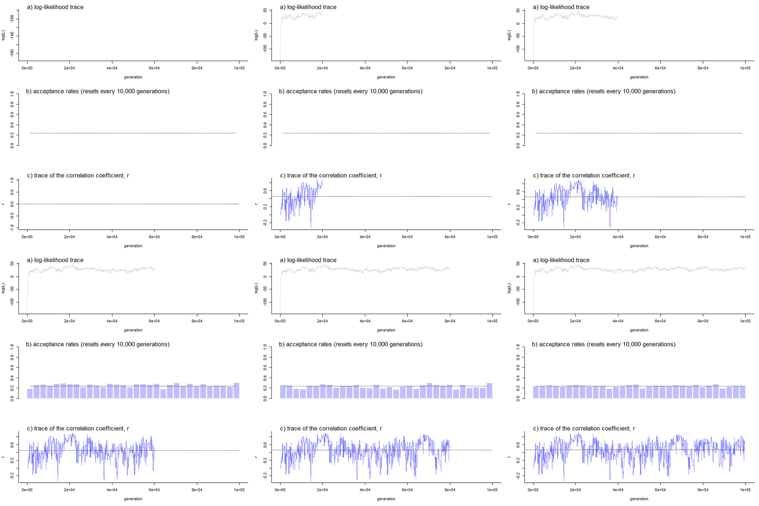
The reason to report (and plot) the acceptance rate is because theory (beyond the scope of this post) tells us that the 'optimal' MCMC acceptance rate is around 0.234. (This makes some sense intuitively - if our acceptance rate is too high or too low our MCMC is very inefficient at sampling from the posterior distribution.) By default threshBayes now auto-tunes its proposal distributions to target an acceptance rate of 0.234.

Note that although the animation is pretty cool, it actually makes threshBayes run a lot slower. A smarter approach is probably just to run the MCMC and then plot a summary afterwards:

plot(sunfish.mcmc)

Finally, let's compute a posterior density for our correlation coefficient between our two traits. Note that because we supplied our binary character as a factor the “direction” of the trait will be in the same order as the levels of the trait.

d<-density(sunfish.mcmc,bw=0.1)
d

## $density
## 
## Call:
##  "density.threshBayes(x = sunfish.mcmc  bw = bw)"
## 
## Data: sunfish.mcmc (800 obs.);   Bandwidth 'bw' = 0.1
## 
##        x                 y            
##  Min.   :-0.6059   Min.   :0.0000815  
##  1st Qu.:-0.1558   1st Qu.:0.0306884  
##  Median : 0.2944   Median :0.2907375  
##  Mean   : 0.2944   Mean   :0.5547941  
##  3rd Qu.: 0.7446   3rd Qu.:1.0728449  
##  Max.   : 1.1947   Max.   :1.6758849  
## 
## $mean.r
## [1] 0.470032
## 
## attr(,"class")
## [1] "density.threshBayes"

plot(d)
title(main=paste("posterior density of correlation",
    "coefficient, r,\nfrom threshold model"),
    font.main=3)

This tells us the piscivory (as opposed to non-piscivory) has a positive evolutionary correlation under the threshold model with PC 1, which (remember) loaded strongly and positively on relative gape width and positively on relative buccal length.

Neat.