Explainer of Γ rate heterogeneity model for phenotypic traits in phytools

This is a bit of an explainer on how to understand the variable-rate model as implemented in the new phytools function fitgammaMk and described recently on this blog (1, 2, 3, 4).

Just as with a variable site-rate model, so common in molecular phylogenetic inference, the underlying concept of this model is not to imagine we can estimate the rate of trait evolution along each edge – but instead to integrate over a distribution of rate variation in which we optimize the shape parameter of the distribution. Of course, since our rate distribution is discrete (the discretized \(\Gamma\), as is typically used in site models), a posteriori we can also compute the marginal likelihoods that each edge is in each state (as I illustrated yesterday).

Although we’ll actually calculate the likelihood using a modification of the pruning algorithm of Felsenstein, we could alternatively conceptualize this computation via an enumeration of all of the possible ways via which the rates might differ between edges – for a given number of rate categories and \(\alpha\) shape parameter of our discretized \(\Gamma\) distribution. This is what I’m going to do here, but remember, this is merely as an illustration of the model (not as a practical procedure for computing the likelihood).

library(phytools)

## Loading required package: ape

## Loading required package: maps

packageVersion("phytools")

## [1] '2.0.11'

We can start with a simple four taxon tree. A rooted, four taxon tree will have a total of six edges.

tree<-read.tree(
  text="((A:6.7,(B:0.9,C:0.9):5.8):3.3,D:10);")
plotTree(tree,direction="upwards")

Now I’m going to assert a trait vector of my character, which (in this instance) I’ll assume is binary.

x<-setNames(c(0,0,1,0),tree$tip.label)
x

## A B C D 
## 0 0 1 0

For our exercise, we’ll further imagine a value of our \(\Gamma\) distribution shape parameter, \(\alpha\), of \(\alpha\) = 0.2.

For real data, of course, this is a parameter we’d estimate from our data & tree – but in this instance, for the purposes of illustrating our model, I’ll just set it.

alpha<-0.2

When discretized (using the median of each interval), this rate distribution looks as follows. (In practice for this model we might choose a larger number of rate categories, as I have done in prior posts.)

nrates<-4 # number of rate categories
r<-qgamma(seq(1/(2*nrates),1,by=1/nrates),
  alpha,alpha)
r<-r/mean(r)
r

## [1] 0.0001436574 0.0350496709 0.4738615302 3.4909451414

To get a matrix giving me all possible combinations of these four different rates across the six edges or branches of my tree, I’ll use the function expand.grid – which is meant (I believe) to be used to generate a design matrix for factorial experiments, but will serve our purposes perfectly well here.

E<-as.matrix(
  expand.grid(replicate(nrow(tree$edge),
  1:nrates,simplify=FALSE)))
head(E,20)

##       Var1 Var2 Var3 Var4 Var5 Var6
##  [1,]    1    1    1    1    1    1
##  [2,]    2    1    1    1    1    1
##  [3,]    3    1    1    1    1    1
##  [4,]    4    1    1    1    1    1
##  [5,]    1    2    1    1    1    1
##  [6,]    2    2    1    1    1    1
##  [7,]    3    2    1    1    1    1
##  [8,]    4    2    1    1    1    1
##  [9,]    1    3    1    1    1    1
## [10,]    2    3    1    1    1    1
## [11,]    3    3    1    1    1    1
## [12,]    4    3    1    1    1    1
## [13,]    1    4    1    1    1    1
## [14,]    2    4    1    1    1    1
## [15,]    3    4    1    1    1    1
## [16,]    4    4    1    1    1    1
## [17,]    1    1    2    1    1    1
## [18,]    2    1    2    1    1    1
## [19,]    3    1    2    1    1    1
## [20,]    4    1    2    1    1    1

Our matrix, E, contains a total of 4,096 (4⁶) rows.

This is the exact number of different ways our four rate categories might be distributed across the six edges of our four taxon tree.

You can already see that for a larger tree or higher number of rate categories the matrix E would become prohibitively large! This is one of the reasons this would not be a practical algorithm for computing the likelihood!

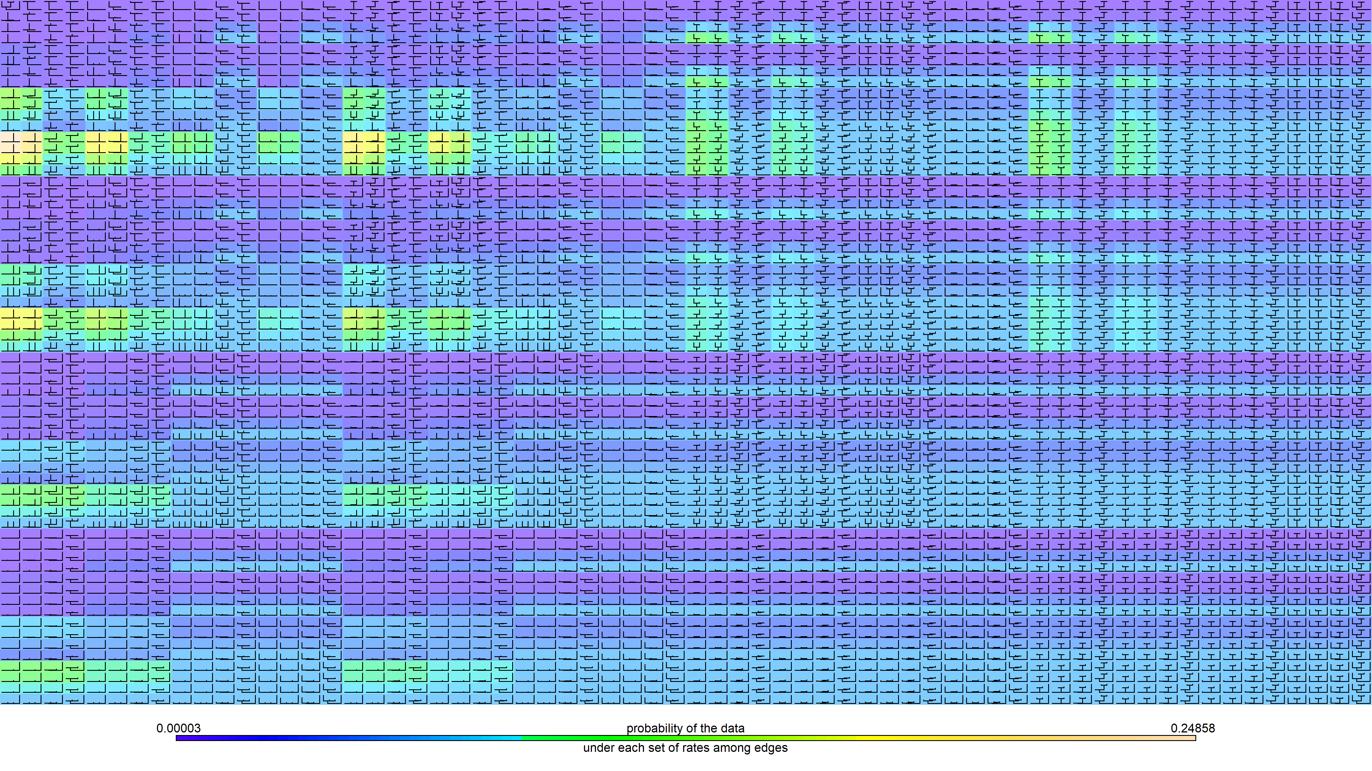
Now, for this demo, I’m going to generate all 4,096 of these rate-varying-trees. I do that by simply multiplying my edge lengths of the original tree by a different set of my discrete \(\Gamma\) rates for each tree.

foo<-function(ind,tree,r){
  tree$edge.length<-tree$edge.length*r[ind]
  tree
}
rate_trees<-apply(E,1,foo,tree=tree,r=r)

Finally, we’ll assume the following simple value of Q (which, once again, in practice we’d co-estimate with \(\alpha\))…

Q<-matrix(c(-1,1,1,-1),2,2,byrow=TRUE,
  dimnames=list(0:1,0:1))
Q

##    0  1
## 0 -1  1
## 1  1 -1

… and then proceed to compute the probability of our tip data on each tree.

lik<-sapply(rate_trees,function(t,x,Q) 
  exp(logLik(fitMk(t,x,fixedQ=Q))),
  x=x,Q=Q)
col_func<-function(x){
  rgb<-colorRamp(topo.colors(n=10))(x)
  make.transparent(
    rgb(rgb[1],rgb[2],rgb[3],maxColorValue=255),0.5)
}
mat<-matrix(c(1:nrow(E),rep(nrow(E)+1,sqrt(nrow(E))*6)),
  sqrt(nrow(E))+6,sqrt(nrow(E)),byrow=TRUE)
layout(mat)
for(i in 1:length(rate_trees)){
  plotTree(rate_trees[[i]],fsize=0.5,lwd=1,plot=FALSE,
    mar=rep(0,4),ylim=c(0,Ntip(tree)+1))
  pp<-get("last_plot.phylo",envir=.PlotPhyloEnv)
  polygon(par()$usr[c(1,2,2,1)],par()$usr[c(3,3,4,4)],
    col=col_func((lik[i]-min(lik))/diff(range(lik))),
    border=FALSE)
  plotTree(rate_trees[[i]],ftype="off",lwd=1,add=TRUE,
    direction="upwards")
}
plot(NA,xlim=c(-1,1),ylim=c(-1,1),mar=rep(0,4),axes=FALSE,
  bty="n")
options(scipen=6)
add.color.bar(1.6,cols=topo.colors(n=100),
  title="probability of the data",lims=range(lik),digits=5,lwd=5,
  subtitle="under each set of rates among edges",prompt=FALSE,
  x=-0.8,y=0,fsize=1.3)

Right-click on image or click here for full size.

(Keep in mind that by exponentiating these values I have a probability, not a log-probability.)

To get the total probability of our data under our model and given our input tree, we assume that each of these different arrangements of the rates across edges are equiprobable a priori and compute their sum, divided by the number of such arrangements that exist! I’ll take the log of that value

log(sum(lik)/length(lik))

## [1] -3.136147

Appropriately, with fitgammaMk we get exactly the same log-likelihood (assuming we fix Q and \(\alpha\), of course).

obj<-fitgammaMk(tree,x,fixedQ=Q,nrates=nrates,
  alpha.init=alpha,marginal=TRUE)

##   --
##   Computing marginal scaled likelihoods (in parallel) of each
##   rate on each edge. Caution: this is NOT fast....
##   --

obj

## Object of class "fitgammaMk".
## 
## Fitted (or set) value of Q:
##    0  1
## 0 -1  1
## 1  1 -1
## 
## Fitted (or set) value of alpha rate heterogeneity
## (with 4 rate categories): 0.2
## 
## Fitted (or set) value of pi:
##   0   1 
## 0.5 0.5 
## due to treating the root prior as (a) flat.
## 
## Log-likelihood: -3.136147 
## 
## Optimization method used was ""

This is good.

Finally, let’s visualize the estimated rates across edges under our model.

plot(obj,outline=TRUE,lwd=5)

Cool. I hope that’s helpful.