Thursday, February 28, 2013

Using bind.tip (or bind.tree) on a tree with node labels

Just a quick point of (searchable) clarification for both phytools bind.tip and the ape function bind.tree (bind.tip, after all, uses bind.tree interally; 1, 2). Regardless of whether or not your tree contains node labels (or tip labels, for that matter), the argument where should give the node number (from the matrix tree$edge), at or below which the tip or subtree should be bound.

Node numbers can be seen using:
plotTree(tree,node.numbers=T)
## OR
plot(tree)
nodelabels() # i.e., no arguments

If you want to bind a new tip or subtree to a terminal edge (i.e., an edge ending with a tip), then the 'node number' is just the index of the species in tree$tip.label. We can get this by (for tip name tip) setting where=which(tree$tip.label==tip). Alternatively, if we want to see the node & tip numbers plotted on the tree we could do:
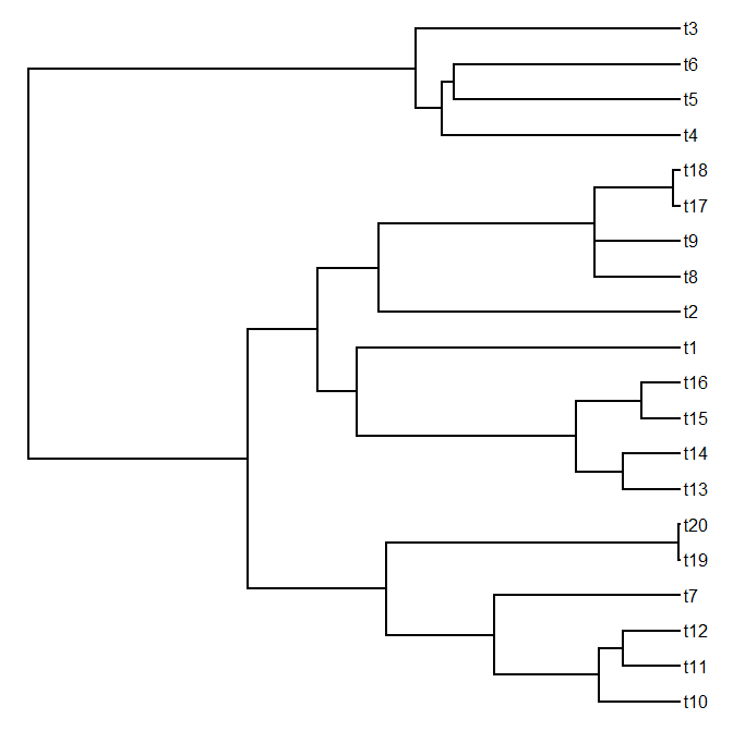
> tree<-pbtree(n=20)
> plot(tree,no.margin=T,label.offset=0.1) # offset may vary
> nodelabels()
> tiplabels()
If adding multiple tips to the tree, remember to keep in mind that each time a new tip is added, the set of node numbers will change. For example:
> tree2<-bind.tip(tree,"t21",where=23,position= 0.5*tree$edge.length[which(tree$edge[,2]==23)])
> ## this just added a new tip halfway along the edge
> ## ending at node 23
> plot(tree2,no.margin=T,label.offset=0.1)
> nodelabels()
> tiplabels()

That's all for now!

Function to count transitions from a mapped tree

To address a user request I just posted a simple function, countSimmap (code here), to count the number of transitions (in total and by type) on a discrete character mapped tree such as a stochastically mapped (i.e., SIMMAP) tree.

Here's a quick demo:
> require(phytools)
> source("utilities.R")
> Q<-matrix(c(-2,1,1,1,-2,1,1,1,-2),3,3)
> colnames(Q)<-rownames(Q)<-c("A","B","C")
> tree<-sim.history(pbtree(n=10,scale=1),Q)
> cols<-setNames(c("blue","red","green"),colnames(Q))
> par(col="white")
> plotTree(tree,ftype="i",lwd=5)
> par(col="black")
> plotSimmap(tree,cols,pts=F,lwd=3,ftype="i",add=T)
> countSimmap(tree,colnames(Q))
$N
[1] 13

$Tr
  A B C
A 0 6 1
B 4 0 2
C 0 0 0

$message
[1] "N is the total number of character changes on the tree"
[2] "Tr gives the number of transitions from row state->column state"

The function is even fast enough to run on quite large trees with lots of transitions, for instance:
> tree<-sim.history(pbtree(n=1000,scale=10),Q)
> system.time(XX<-countSimmap(tree,colnames(Q)))
  user  system elapsed
  0.22    0.00    0.22
> XX
$N
[1] 3762

$Tr
   A   B   C
A   0 623 646
B 605   0 623
C 656 609   0

$message
[1] "N is the total number of character changes on the tree"
[2] "Tr gives the number of transitions from row state->column state"

That's it.

Wednesday, February 27, 2013

New phytools build and rep() function for "phylo" objects

I just posted a new minor version of 'phytools' (phytools 0.2-22). You can download it here, and install from source.

Relative to the last minor version, this version has only the new function writeAncestors, as well as a function called internally by writeAncestors called repPhylo. repPhylo merely does what the 'base' function rep does for vectors and lists, but for "phylo" objects. This turned out to be annoyingly difficult, until I realized that I could work from this solution on stackoverflow.com.

Here it is, modified for "phylo" objects:
repPhylo<-function(tree,times){
 tree<-
 if(sum(sapply(tree,class)!="list")==0){
   tree
 } else {
     list(tree)
 }
 tree<-rep(tree,length=times)
 class(tree)<-"multiPhylo"
 return(tree)
}

New function to write trees with ancestral states and CIs

A phytools user today requested the ability to output ancestral state estimates (and confidence intervals) to file within a Newick string. Specifically, he had the following suggestion:

It would be great if we could get the ancestral state values as well as the 95CI written in the same tree. So perhaps it is possible to append multiple values to the node like beast does with the 95HPD for divergence time estimates. I looked at the format and it puts multiple values after a node like this [&CI={lower 95%, upper 95%}, ancstate={value}].

Theoretically, this should be straightforward using the optional "phylo" attribute node.label. We could just do, for example:
> tree<-pbtree(n=10)
> x<-fastBM(tree)
> XX<-fastAnc(tree,x,CI=T)
> XX<-lapply(XX,round,2)
> tree$node.label<-paste("[&CI={",XX$CI95[,1],",", XX$CI95[,2],"},ancstate={",XX$ace,"}]",sep="")
> write.tree(tree,digits=2)
[1] "(t1:1.5,(((((t9:0.15,t10:0.15)[&CI={1.061.75}ancstate={1.4}]:0.15,t6:0.3)...

Oops. Unfortunately, this didn't work because write.tree has dropped all of our commas from node.label, even when they're within [...] square parentheses! This is presumably by design to prevent us from using Newick only characters in node labels, although they will be ignored by convention by most applications if given within square brackets.

Luckily, I already have code for tree writing in the form of the phytools function write.simmap, and I thought (rightfully) that it wouldn't be too difficult to modify the code of this function to be able to include ancestral state estimates and CIs in the requested manner.

Well, I ended up building a much more versatile function than I originally intended. writeAncestors (code here) can write trees with ancestors and CIs in "phylip" (i.e., simple Newick) or "nexus" format; it can accept as input the results from ace or fastAnc, and it detects automatically whether or not CIs should be included. In the event that a data vector is provided (that is, tip data instead of the inferred states at nodes) writeAncestors will estimate ancestral states and (optionally) CIs assuming Brownian evolution using fastAnc. In the event that multiple trees, sets of ancestral states, or data vectors are provided, writeAncestors will try to act appropriately.

Here's a quick demo of its simplest usage (some output omitted):
> ls()
[1] "tree" "x"    "XX"  
> source("writeAncestors.R")
> args(writeAncestors)
function (tree, Anc = NULL, file = "", digits = 6,
   format = c("phylip", "nexus"), ...)
NULL
> writeAncestors(tree,XX,digits=2)
(t1:1.47,(((((t9:0.15,t10:0.15)[&CI={1.06,1.75},ancstate={1.4}]:0.15,t6:0.3)...
> # now with a data vector as input
> writeAncestors(tree,x=x,digits=3)
(t1:1.468,(((((t9:0.153,t10:0.153)[&CI={1.057,1.752},ancstate={1.405}]:0.148,t6:0.301)...
> # now to Nexus file (we'll output to screen)
> writeAncestors(tree,x=x,format="nexus")
#NEXUS
[R-package PHYTOOLS, Wed Feb 27 15:47:46 2013]

BEGIN TAXA;
       DIMENSIONS NTAX = 10;
       TAXLABELS
               t1
               t10
               ...
       ;
END;
BEGIN TREES;
       TRANSLATE
               1       t1,
               2       t10,
   ...
       ;
       TREE * UNTITLED = [&R] (1:1.467541,(((((10:0.153423,2:0.153423)[&CI={1.05681,1.75229},ancstate={1.40455}]...
END;

Well, that's it.

Tuesday, February 26, 2013

On the shape of trees with random taxa addition or subtraction

Since I have a new function for add tips at random to a tree; and it is even easier to write a function to drop tips randomly from the tree - i.e., here it is:
drop.random<-function(tree,n=1)
   tree<-drop.tip(tree,tip=sample(tree$tip.label)[1:n])
I thought it might be fun to look at the effects of adding or subtracting tips at random from the tree. We already know that random missing taxa tends to create trees with longer than expected terminal edges - seemingly a slow-down in the rate of lineage diversification through time.

This is not very scientific, but first let's look at the LTT and Pybus & Harvey's (2000) γ for a single tree that we initiate with 100 species and then add to randomly using add.random in increments of 10. Here's our code (minus creating the video):
require(phytools)
tree<-pbtree(n=100,scale=1)
mas<-900
for(i in 1:(mas/10+1)){
  x<-ltt(tree,plot=FALSE)
  plot(x$times[2:length(x$times)],x$ltt[2:length(x$ltt)], xlab="time",ylab="lineages",log="y",type="l",xlim=c(0,1), ylim=c(2,max(x$ltt)))
  lines(c(0,1),c(2,max(x$ltt)),lty=2)
  text(x=0,y=max(x$ltt),paste("N = ",length(tree$tip), "\n","gamma = ",round(x$gamma,3),sep=""),adj=c(0,1))
  tree<-add.random(tree,n=10)
}

And here's the result:

OK, next, let's do the opposite - start with 1000 taxa and drop taxa random. First the code:
drop.random<-function(tree,n=1)    tree<-drop.tip(tree,tip=sample(tree$tip.label)[1:n])
require(phytools)
tree<-pbtree(n=1000,scale=1)
menos<-900
for(i in 1:(menos/10+1)){
x<-ltt(tree,plot=FALSE)
  plot(x$times[2:length(x$times)],x$ltt[2:length(x$ltt)],xlab="time", ylab="lineages",log="y",type="l",xlim=c(0,1), ylim=c(2,max(x$ltt)))
  lines(c(0,1),c(2,max(x$ltt)),lty=2)
  text(x=0,y=max(x$ltt),paste("N = ",length(tree$tip), "\n","gamma = ",round(x$gamma,3),sep=""),adj=c(0,1))
  tree<-drop.random(tree,n=10)
}

And the video:

Adding taxa at random, at least by our algorithm, does not seem to affect tree shape all that much; but subtracting random tips, as we expected, makes γ turn progressively more and more negative.

To see if this is idiosyncratic to the specific trees we started with, why don't we replicate the entire process (i.e., 900% addition or subtraction) in a single step for, say, 30 random pure-birth trees. Here's what that looks like. First, adding tips randomly:
XX<-matrix(NA,31,2,dimnames=list(NULL,c("gamma100","gamma1000")))
require(phytools)
for(i in 1:31){
  tree<-pbtree(n=100)
  XX[i,1]<-ltt(tree,plot=F)$gamma
  tree<-add.random(tree,900)
  XX[i,2]<-ltt(tree,plot=F)$gamma
}
colMeans(XX)
ZZ<-hist(XX[,2]-XX[,1],plot=F,breaks=-9.5:0.5)
barplot(ZZ$density,names=ZZ$mids,space=0,main=expression(gamma[100]-gamma[1000]))

And the results:
> colMeans(XX)
 gamma100  gamma1000
0.3568899 -1.9163830
And if we do the same thing dropping tips, here are the results:
> colMeans(YY)
 gamma100  gamma1000
-6.1072618 0.2275565
So, on the face of it, it seems as though adding taxa randomly (from 100 to 1000 species in the tree) or dropping taxa (from 1000 to 100) both result in a decrease in γ - however the scale of decrease is highly asymmetrical, with random subtraction resulting in a much greater decrease in γ.

At the start of this little experiment I wasn't sure if random addition of taxa would increase or decrease γ, and in the end it seems to decrease γ but sometimes only a little.

New version of package for numerical analyses in evolutionary biology

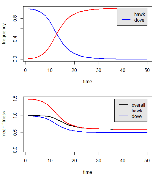
I just added a new function to my little R package 'popgen' for numerical analyses and simulation in evolution and population genetics (see my previous post on this here). The function is called hawk.dove and does numerical analysis of a simple discrete-time hawk-dove model. It then shows the result in a two panel plot. The first panel gives the frequencies of each phenotype through time; whereas the second plot gives the mean fitness of the population and the mean fitness of each strategy. The idea is to play with the payoff matrix to see how the behavior of the model changes. Coexistence of both hawk and dove strategies, or extinction of one or the other, are all possible.

Here's a demo. First download the package source (popgen 0.2).

> install.packages("popgen_0.2.tar.gz",type="source", repos=NULL)
...
* DONE (popgen)
> payoff<-matrix(c(0.6,1.5,0.5,1.0),2,2,byrow=T)
> colnames(payoff)<-rownames(payoff)<-c("hawk","dove")
> payoff
    hawk dove
hawk  0.6  1.5
dove  0.5  1.0
> hawk.dove(M=payoff,time=50)
Pay-off matrix:
    hawk dove
hawk  0.6  1.5
dove  0.5  1.0

That's it.

Monday, February 25, 2013

More on 'untangling' misplotted trees

I just posted a new function, untangle, which attempts to "untangle" branch crossing resulting from bind.tree or other functions.

It has two different methods: method="reorder" and method="read.tree" (as described here), and will also attempt to untangle SIMMAP style trees automatically using reorderSimmap. I've included it in a non-CRAN version of phytools (phytools 0.2-21), which can be downloaded from the phytools website and installed from source. This version also includes an updated version of phenogram.

Here's a quick demo of untangle with SIMMAP style trees:
> install.packages("phytools_0.2-21.tar.gz",type="source", repos=NULL)
...
* DONE (phytools)
> require(phytools)
Loading required package: phytools
> tree<-add.random(pbtree(n=5),n=45)
> Q<-matrix(c(-1,1,1,-1),2,2)
> rownames(Q)<-colnames(Q)<-c(1,2)
> cols<-setNames(c("blue","red"),c(1,2))
> mtree<-sim.history(tree,Q,anc="1")
> plotSimmap(mtree,cols,pts=F,lwd=3)
> mtree<-untangle(mtree)
> plotSimmap(mtree,cols,pts=F,lwd=3)

That's it.

'Tangled trees' from add.random

Today I received the following bug report about the relatively new phytools function add.random:

I had a question about the add.random function you posted on your phytools blog a few weeks ago. Occasionally when I add a set of tips, the resulting phylogeny plots so that some branches cross. Anecdotally, it seems to happen only (or at least more often) when the number of added tips > number of ‘real’ tips in the tree (but I haven’t looked at this much). The phylo.object seems to function as I’d expect otherwise so it seems to just be a plotting thing, but I don’t know enough about how plot.phylo reads the phylo object to know for sure.

Indeed this bug is quite easy to replicate:
> set.seed(6)
> tree<-pbtree(n=5)
> treeAdded<-add.random(tree,n=10)
> layout(c(1,2))
> plotTree(tree); plotTree(treeAdded)

Obviously, there is branch crossing here. I'm going to pass the buck a bit here and mention that although add.random calls the phytools function bind.tip (1,2) internally, bind.tip is little more than a thinly coded wrapper for the 'ape' function bind.tree.

Branch crossing appears to occasionally occur because both plot.phylo (in ape) and plotTree (in phytools) assume a particular ordering for the edges and tips in tree$edge, which sometimes fails to be satisfied when a lot of tips have been added to the tree. Luckily, this only affects plotting (so far as I know), and none of the other functions of the "phylo" object.

Fortunately, this is also incredibly easy to solve. The following are two different functions that will "untangle" the tree, so to speak:

untangle1<-function(x) reorder(reorder(x,"pruningwise"))
## or
untangle2<-function(x) read.tree(text=write.tree(x))

We can try it out on our previous example, from above:
> treeUntangled1<-untangle1(treeAdded)
> treeUntangled2<-untangle2(treeAdded)
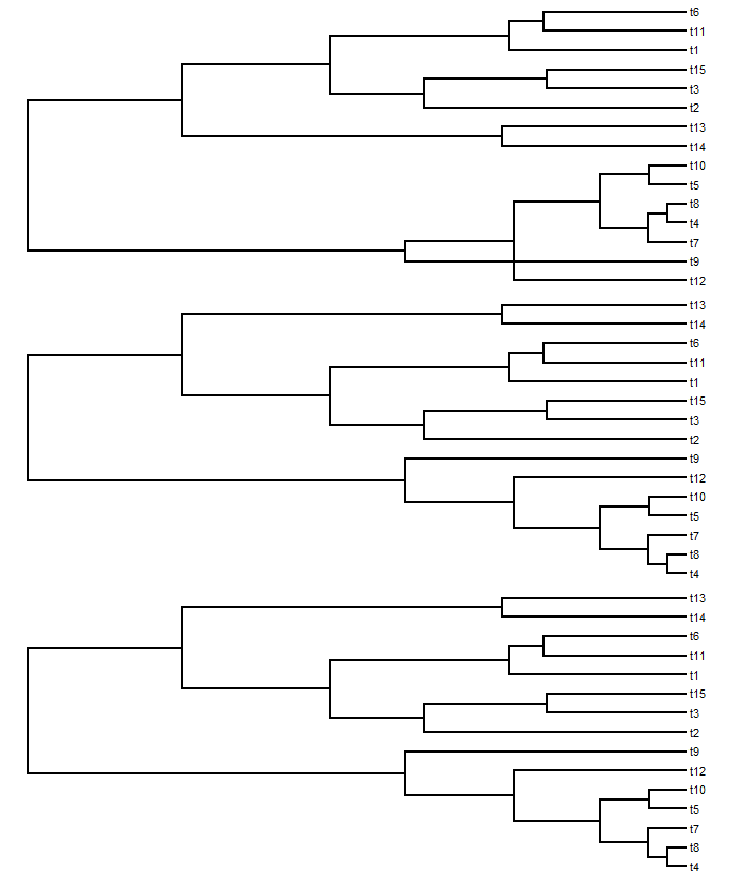
> layout(c(1,2,3))
> plotTree(treeAdded)
> plotTree(treeUntangled1)
> plotTree(treeUntangled2)

Since both functions do the job, we can also ask if one is more computationally efficient than the other. Let's do this using a much bigger tree. We'll do that using system.time:
> tree<-pbtree(n=5)
> # this takes a while!
> tree<-add.random(tree,n=2000)
> plotTree(tree,ftype="off",lwd=1)
> # lots of tangles!
> system.time(tree1<-untangle1(tree))
  user  system elapsed
     0       0       0
> system.time(tree2<-untangle2(tree))
  user  system elapsed
  0.37    0.00    0.37
> plotTree(tree1,ftype="off",lwd=1)
> # untangled! (tree2 is the same)
> all.equal(tree,tree1)
[1] TRUE
> all.equal(tree,tree2)
[1] TRUE

It's a small difference, but the reorder.phylo method is lightning fast! One important note - users should be aware that the tip & node numbers of our tree change when we untangle it.

That's it. I will write a new utility function, untangle, that will do this and also untangle SIMMAP style "phylo" objects. When I get around to that, I'll post it.

Thursday, February 21, 2013

Type I error and power of the 'phylogenetic ANOVA'

There are a couple of different statistical methods that are commonly referred to as the phylogenetic ANOVA.

The phylogenetic ANOVA is generally meant to refer to the simulation approach of Garland et al. (1993). Under this method, we fit the ANOVA model in the typical way - but then we conduct Brownian numerical simulations on the tree to obtain a null distribution of the model test statistic (F). This Monte Carlo simulated null distribution is used for hypothesis testing. The Garland et al. (1993) phylogenetic ANOVA is implemented in the function phy.anova from the geiger package, as well as in the phytools function phylANOVA, which adds post-hoc tests.

The second approach is what I'm going to refer to as the phylogenetic generalized least squares (GLS) ANOVA. Under this model we used the mechanics of GLS to fit a linear model in which the residual error of the model has phylogenetic autocorrelation. This is analogous, and mathematically equivalent, to fitting a phylogenetic regression (sensu Grafen 1989), as described in Rohlf (2001).

The disadvantage of the former approach is that it cannot be used to estimate the coefficients of the fitted ANOVA model - only the p-value of this fit. This is because the OLS estimators (although statistically unbiased) are not minimum variance - and may have very high variance (probably depending on the phylogenetic structure of the independent variable). By contrast, GLS has the advantage of giving unbiased and minimum variance estimators of the fitted model coefficients - that is, conditioned on our model for the residual error being correct.

In spite of the similarity of the goals of these two different approaches, to my knowledge no prior study has compared their type I error or power. The code below can be used to estimate the type I error of each approach, as well as standard OLS (i.e., ignoring the phylogeny):

# load required packages
require(phytools)
require(nlme)

# number of replicates
N<-200

# balanced tree
tree<-compute.brlen(stree(n=128,type="balanced"))

# transition matrix for simulation
Q<-matrix(c(-2,1,1,1,-2,1,1,1,-2),3,3)
rownames(Q)<-colnames(Q)<-c(0,1,2)

# simulate discrete character
mtrees<-replicate(N,sim.history(tree,Q),simplify=FALSE)
class(mtrees)<-"multiPhylo"

# plot (just for fun)
cols<-c("white","blue","red"); names(cols)<-0:2
foo<-function(x){
  plotTree(x,ftype="off",lwd=5)
  plotSimmap(x,cols,pts=FALSE,ftype="off",lwd=3,add=TRUE)
}
lapply(mtrees,foo)

# conduct simulations under the null
anovaOLS<-anovaPGLS<-anovaGarland<-list()
for(i in 1:N){
  b<-c(0,0,0)
  x1<-factor(mtrees[[i]]$states,levels=c(0,1,2))
  e<-fastBM(mtrees[[i]])
  y<-as.vector(b%*%t(model.matrix(~0+x1))+e)
  anovaOLS[[i]]<-anova(gls(y~x1,data.frame(y,x1)))
  anovaPGLS[[i]]<-anova(gls(y~x1,data.frame(y,x1), correlation=corBrownian(1,mtrees[[i]])))
  anovaGarland[[i]]<-phylANOVA(mtrees[[i]],x1,y,posthoc=F)
  print(paste("replicate",i))
}

# extract the p-values of the fitted models
pOLS<-sapply(anovaOLS,function(x) x$'p-value'[2])
pGLS<-sapply(anovaPGLS,function(x) x$'p-value'[2])
pGarland<-sapply(anovaGarland,function(x) x$Pf)

From here it is simple to get the type I error rate for each method:
> # get type I error
> typeI.OLS<-mean(pOLS<=0.05)
> typeI.GLS<-mean(pGLS<=0.05)
> typeI.Garland<-mean(pGarland<=0.05)
> typeI.OLS
[1] 0.85
> typeI.GLS
[1] 0.04
> typeI.Garland
[1] 0.06

So, it looks like Garland et al.'s simulation method and phylogenetic GLS both have appropriate type I error rates when there is no effect of the independent variable - but ignoring the phylogeny entirely can result in very high type I error. I should note that the simulation approach - using phylogenetic simulation of x and Grafen's branch lengths - is kind of the "worst case scenario" for ignoring phylogeny.

We can loop around this code and ask whether the power to detect an effect of various sizes differs between PGLS-ANOVA and Garland et al.'s simulation approach. Here is the code I used as well as the result. To be able to run through this a little quicker, I decided to use only the first 100 trees from my prior simulation.

# power analysis
N<-100
power.GLS<-typeI.GLS; power.Garland<-typeI.Garland
anovaPGLS<-anovaGarland<-list()
for(i in 1:10){
  for(j in 1:N){
    # simulate an effect
    # note that this relative to a variance between tips
    # separated by the root of 1.0
    b<-c(0,-0.1*i,0.1*i)
    x1<-factor(mtrees[[j]]$states,levels=c(0,1,2))
    e<-fastBM(mtrees[[j]])
    y<-as.vector(b%*%t(model.matrix(~0+x1))+e)
    anovaPGLS[[j]]<-anova(gls(y~x1,data.frame(y,x1), correlation=corBrownian(1,mtrees[[j]])))
    anovaGarland[[j]]<-phylANOVA(mtrees[[j]],x1,y, posthoc=F)
    print(paste("effect",i*0.1,"- replicate",j))
  }
  # extract the p-values of the fitted models
  pGLS<-sapply(anovaPGLS,function(x) x$'p-value'[2])
  pGarland<-sapply(anovaGarland,function(x) x$Pf)
  # get power
  power.GLS[i+1]<-mean(pGLS<=0.05)
  power.Garland[i+1]<-mean(pGarland<=0.05)
}
plot(0:10/10,power.GLS,type="b",ylim=c(0,1), xlab="effect size",ylab="power")
lines(0:10/10,power.Garland,type="b")
lines(c(0,1),c(0.05,0.05),lty=2)
text(x=1,y=0.95,"PGLS",pos=2,offset=0)
text(x=1,y=0.7,"Garland et al.",pos=2,offset=0)
So, there you have it. If I've done this properly, it suggests that the Garland et al. simulation method has the correct type I error - but relatively low power compared to PGLS. Cool.

One caveat that I'd like to attach to all of this is that I've always found the presumed generating process - one in which the mean structure effectively evolves 'saltationally' (changing state spontaneously whenever the discrete character changes state) but the error structure evolves by Brownian evolution - to feel more than a little artificial.

That being said, I still feel that this result might interest some people. Could this be a published 'note?' I'm not sure, but feedback is welcome.

Monday, February 18, 2013

Visualizing uncertainty in a 'traitgram'

For a variety of a reasons, I've been thinking about clever ways to try and visualize uncertainty in ancestral state estimates. Here is one attempt using an adaptation of the phytools function phenogram. This function plots a projection of the tree into a two dimensional space defined by time since the root (on the x) and phenotype. Note that to run this I had to first add the optional argument add to phenogram, so you will need to download and load the source (phenogram.R) to get this to work.

library(phytools)
# load source
source("phenogram.R")
# simulate tree & data
tree<-pbtree(n=20)
plotTree(tree)
x<-fastBM(tree)
# estimate ancestors
A<-fastAnc(tree,x,CI=TRUE)
tree<-paintSubTree(tree,node=length(tree$tip)+1,"1")
# our transparencies
trans<-as.character(floor(0:50/2))
trans[as.numeric(trans)<10]<-
  paste("0", trans[as.numeric(trans)<10],sep="")
# plot
for(i in 0:50){
  p<-i/length(trans)
  phenogram(tree,c(x,(1-p)*A$CI95[,1]+p*A$ace), colors=setNames(paste("#0000ff",trans[i+1],sep=""),1), add=i>0)
  phenogram(tree,c(x,(1-p)*A$CI95[,2]+p*A$ace), colors=setNames(paste("#0000ff",trans[i+1],sep=""),1), add=TRUE)
}
phenogram(tree,c(x,A$ace),add=TRUE, colors=setNames("white",1))
One word of caution about this visualization. Since I plot uncertainty using transparent colors, it can be difficult to impossible to extract uncertainty about any specific ancestral node from this plot. However what the plot is good at showing is the probability density of all hypothetical ancestors at any time slice through the tree.

Sunday, February 17, 2013

New version of phytools on CRAN (phytools 0.2-20)

A new version of phytools (phytools 0.2-20) is now on CRAN. Presently you can download the source code for this version from the phytools homepage or phytools CRAN page and install from source. Windows and Mac OS binaries should be built soon and eventually these will percolate through all the different CRAN mirrors.

Due to updates in a couple of different functions, phytools now depends on ape ≥ 3.0-7 (the latest version of ape as of the present date) and imports from phangorn ≥ 1.6-3.

Here's a brief list of some of the updates in phytools 0.2-20 relative to the last CRAN version (0.2-1):

1. A new function, splitplotTree, to plot a phylogeny in multiple columns or plotting windows.

2. A new function, bind.tip, for adding a single tip to the tree (1, 2).

3. A couple of critical bug fixes for phyl.RMA (1, 2).

4. A significant update to the function matchNodes which matches nodes between trees based either on the descendant tips from each node or on the distances from nodes to the tips in the tree.

5. A new utility function, applyBranchLengths, which applies the branch lengths from one tree to other topologically identical phylogenies.

6. New versions of ancThresh (e.g., here) and user control of phytools function plotThresh and threshDIC.

7. A new function, add.random, to add tips at random to a phylogeny.

8. An important update to pgls.Ives, to accept individual data, rather than just species means and standard errors.

9. A new function, orderMappedEdge, to reorder the "phylo" object mapped.edge in SIMMAP style trees.

10. A new version of the function, mrp.supertree, for MRP supertree estimation (1, 2).

11. Update to the function phylANOVA for phylogenetic ANOVA based on Garland et al. (1993).

12. A new version of fastAnc to compute the variances and 95% CIs on ancestral states.

13. A new function, getSisters, to get the node(s) or tip(s) that are sister to a focal node.

14. Minor updates to several functions including add.everywhere, allFurcTrees, anc.Bayes, anc.ML, anc.trend, ancThresh, brownie.lite, estDiversity, evol.rate.mcmc, evol.vcv, evolvcv.lite, exhaustiveMP, fancyTree, fitBayes, make.simmap, optim.phylo.ls, phyl.pairedttest, phylomorphospace, plotSimmap, reroot, sim.corrs, sim.history, sim.rates, and write.simmap.

15. Finally, as I mentioned before, a change in the dependency relationship with ape and phangorn. phytools now depends on ape ≥ 3.0-7 - but imports from phangorn (≥ 1.6-3).

Friday, February 15, 2013

Function to get the sister(s) of a node or tip

I just posted a new utility function, getSisters, that takes as input a tree and a node or tip number or label, and returns the sister node or tip numbers or labels. It has two modes: mode="number", which returns node or tip numbers as an integer or vector; and mode="label" which returns a list with up to two components - one component for node labels (if available) or numbers, and the other component with tip labels.

The code for the function is here, but it also in the most recent build of phytools: phytools 0.2-18.

Here's a quick demo:
> require(phytools)
> tree<-rtree(n=12)
> plotTree(tree,node.numbers=TRUE)
> getSisters(tree,19)
[1] 23
> getSisters(tree,18,mode="label")
$tips
[1] "t10"

You get the idea. We can also collapse some branches so that some tips or nodes have multiple sister tips or nodes:
> tree$edge.length[which(tree$edge[,2]==18)]<-0
> tree$edge.length[which(tree$edge[,2]==23)]<-0
> tree$edge.length[which(tree$edge[,2]==20)]<-0
> tree$edge.length[which(tree$edge[,2]==21)]<-0
> tree<-di2multi(tree)
> plotTree(tree,node.numbers=T)
> getSisters(tree,18,mode="label")
$tips
[1] "t8" "t2" "t10"

> getSisters(tree,"t4",mode="label")
$nodes
[1] 19

$tips
[1] "t3" "t11"

That's it.

Thursday, February 14, 2013

New version of fastAnc; new build of phytools

I just posted a new version of the function fastAnc for (relatively) fast ancestral character estimation. The function is previously described here. The main addition to this new version is that now the function (optionally) computes the variance on the ancestral state estimates based on equation (6) of Rohlf (2001), as well as (optionally) 95% confidence intervals on the states. The updated code is here; however, I have also posted a new build of phytools - which can be downloaded here and installed from source.

Note that equation (6) of Rohlf (2001) only gives the relative variance on the ancestral state estimate at the root node. To scale that estimate to our data, we need to multiply by the phylogenetic variance for our continuous trait. This can be computed as the mean square of the contrasts. Once we have the variances, we can compute our 95% CIs on the estimates as the estimates +/- 1.96 × the square root of the variances.

I didn't realize this when I was writing the function, but it turns out to be the case that this update to fastAnc depends on ape >= 3.0-7 (i.e., the newest version of ape as of the date of writing). This is because the options in the ape function for independent contrasts, pic, were expanded in the latest release to include the option of returning the tree with branches scaled to expected variance - which we can conveniently exploit to do the calculation of equation (6) in Rohlf.

I should also point out that the 95% CIs obtained by this function differ in a substantial way from the 95% CIs computed in ace. Specifically, the 95% CIs computed in ace would seem to be too small. We can show this relatively easily by simulation, as follows:

> onCI.ace<-onCI.fastAnc<-vector()
> N<-100
> for(i in 1:1000){
+ tree<-pbtree(n=N)
+ x<-fastBM(tree,internal=TRUE)
+ a<-fastAnc(tree,x[1:N],vars=TRUE,CI=TRUE)
+ onCI.fastAnc[i]<-sum((x[1:tree$Nnode+N]>a$CI95[,1])*(x[1:tree$Nnode+N]< a$CI95[,2]))/tree$Nnode
+ b<-ace(x[1:N],tree,CI=TRUE)
+ onCI.ace[i]<-sum((x[1:tree$Nnode+N]>b$CI95[,1])*(x[1:tree$Nnode+N]< b$CI95[,2]))/tree$Nnode
+ }
There were 24 warnings (use warnings() to see them)
> warnings()
Warning messages:
1: In sqrt(diag(solve(h))) : NaNs produced
2: In sqrt(diag(solve(h))) : NaNs produced
3: ...
> # this should be 0.95
> mean(onCI.fastAnc)
[1] 0.9483737
> mean(onCI.ace,na.rm=TRUE)
[1] 0.6738759

This simulation shows that although our 95% CIs computed in fastAnc include the generating values almost exactly 95% of the time (94.8% across 1000 simulations with 99 estimated ancestral states per simulation), ace CIs only include the generating value about 67% of the time.

I'm not exactly sure why this is the case, but my best guess is based on the warnings which tell us that the Hessian is being used to compute the standard errors of the parameter estimates and thus the CIs. This is an asymptotic property of the likelihood surface, and for finite sample this approximation can be quite bad (as we see above).

Tuesday, February 12, 2013

Fix to fastAnc

A colleague recently reported bad behavior in the fast ancestral character estimation function fastAnc that he hypothesized was due to the fact that I extracted the total number of tips in the tree using the shorthand N<-length(tree$tip) in place of N<-tree$tip.label. In principle this shouldn't be a problem because list elements, unlike variables, can be called by any unambiguous abbreviation of the element name (that is, if we use the $ operator - see below).

So, for instance:
> exampleList<-list(x=c(1,2),test=c("A","B","C"))
> exampleList$t
[1] "A" "B" "C"
> exampleList$test2<-c("D","E","F")
> exampleList$t # no longer umambiguous
NULL
> exampleList$test
[1] "A" "B" "C"

As an aside, if we want to call elements in a list accepting only an exact match the name, then we have to use [[ instead of $. So, for instance:
> exampleList$test2<-NULL
> exampleList$t
[1] "A" "B" "C"
> exampleList[["t"]]
NULL
> exampleList[["test"]]
[1] "A" "B" "C"
> # tell R to allow partial match
> exampleList[["t",exact=FALSE]]
[1] "A" "B" "C"

This is the reason why either:
> tree<-pbtree(n=112)
> length(tree$tip)
[1] 112
> # or
> length(tree$tip.label)
[1] 112
will, generally speaking, serve equally well in computing the number of tips in a tree.

However, what the exercise above inadvertently shows is that if we were to create a custom "phylo" object (which we have every right to do), we could do so by adding an additional list component, for instance $tip.states. If we did, it could create confusion when we compute the number of terminal species in the tree using length(tree$tip). So, for instance:
> x<-fastBM(tree)
> tree$tip.states<-x
> length(tree$tip)
[1] 0
> length(tree$tip.label)
[1] 112

This suggests that it might not be the best programming practice to assume that length(tree$tip) will invariably compute the number of species in the tree. I have updated fastAnc, here, but I know for a fact that this kind of code shorthand exists in other functions of the phytools package as well. I will try to update these as time goes on.

BTW - in that example with the custom element $tip.states, here is what fastAnc does:
> fastAnc(tree,x)
Error in root(btree, node = i) :
 incorrect node#: should be greater than the number of taxa
> # load the updated source
> source("fastAnc.R")
> fastAnc(tree,x)
       113         114         115  ...
-0.59341281 -0.03688321  0.89743347  ...

Monday, February 11, 2013

Updated phylANOVA

A user phytools user recently contacted me with the bug report that for a tree with multifurcations they received the following error from the function phylANOVA:
Error in pic(y, tree) : 'phy' is not rooted and fully dichotomous

phylANOVA is a function that does the simulation-based phylogenetic ANOVA of Garland et al. (1993), but with posthoc tests about the group means - also based on simulation. (Note that this is the same as the "geiger" function phy.anova, but with the posthoc comparison of means added in.)

There's no inherent reason why the function should require a fully bifurcating tree. The reason that it does is because I use pic as a quick way to compute the Brownian motion rate of evolution for simulation, and pic needs a binary tree as input. This bug is easily fixed.

I've updated the code. The link to the new code is here. The following shows a simulation of a tree with multifurcations and data for the phylogenetic ANOVA; a failed analysis with the current version of the code; and a successful analysis with the updated version. Note that there are some neat tricks of simulation thrown in here....

> # load phytools
> require(phytools)
> # simulate tree
> tree<-pbtree(n=50)
> # set some branches to zero to create polytomies
> tree$edge.length[tree$edge.length<0.1]<-0
> is.ultrametric(tree) # check if ultrametric
[1] FALSE
> # now add some length to terminal branches so that
> # the tree is ultrametric
> addTip<-max(vcv(tree))-diag(vcv(tree))
> tree$edge.length[tree$edge[,2]<=length(tree$tip)]<- tree$edge.length[tree$edge[,2]<=length(tree$tip)]+addTip
> tree<-di2multi(tree)
> is.ultrametric(tree) # check if ultrametric
[1] TRUE
> is.binary.tree(tree) # check if bifurcating
[1] FALSE
> # let's take a look at our tree with polytomies
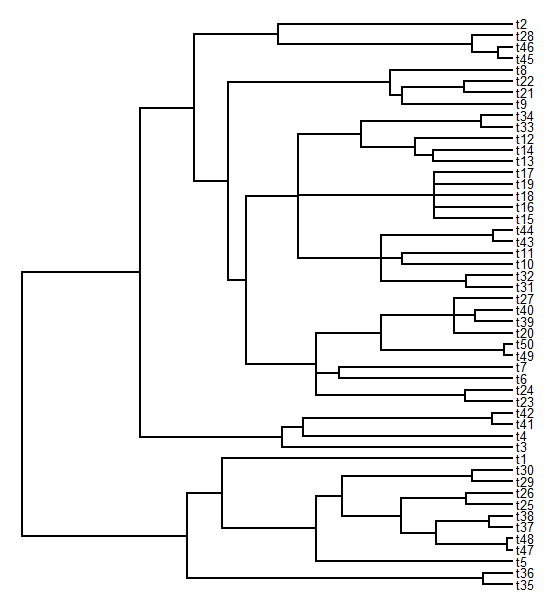
> plotTree(tree,fsize=0.8)
> # ok now let's create a discrete character on the tree
> Q<-matrix(c(-2,1,1,1,-2,1,1,1,-2),3,3)
> rownames(Q)<-colnames(Q)<-c("A","B","C")
> x<-sim.history(tree,Q)$states
> # now let's add an effect that depends on the tip state
> # for the discrete trait
> X<-sapply(c("A","B","C"),"==",x)*1
> y<-X%*%c(0,2,6)+fastBM(tree)
> # conduct phylogenetic ANOVA (current function)
> phylANOVA(tree,x,y) # fails
Error in pic(y, tree) : 'phy' is not rooted and fully dichotomous
> # with a multi2di resolved tree
> phylANOVA(multi2di(tree),x,y)
$F
[1] 10.11326
$Pf
[1] 0.003
$T
        A         B         C
A 0.000000 -1.514359 -4.496845
B 1.514359  0.000000 -2.618537
C 4.496845  2.618537  0.000000
$method
[1] "holm"
$Pt
     A     B     C
A 1.000 0.185 0.003
B 0.185 1.000 0.006
C 0.003 0.006 1.000

> # load updated version
> source("phylANOVA.R")
> phylANOVA(tree,x,y)
$F
[1] 10.11326
$Pf
[1] 0.001
$T
        A         B         C
A 0.000000 -1.514359 -4.496845
B 1.514359  0.000000 -2.618537
C 4.496845  2.618537  0.000000
$method
[1] "holm"
$Pt
     A     B     C
A 1.000 0.172 0.003
B 0.172 1.000 0.014
C 0.003 0.014 1.000

Saturday, February 9, 2013

More on MRP supertree estimation in phytools

In a post from earlier today, I described some of the updates in a new version of the phytools function mrp.supertree. The two main changes are as follows: (1) now the user can decide which parsimony optimization method (optim.parsimony or pratchet) is called inside the function; and (2) now near total control of the optimizer has been transferred to the user.

What this means is that (with one exception*) all the options of optim.parsimony and pratchet (summarized here) can now be controlled by the user. The exception is really only a modification to how the optimizer is controlled. For mrp.supertree(...,method="optim.parsimony") the argument start is substituted for the argument tree in optim.parsimony; and, for both mrp.supertree(...,method="pratchet") and mrp.supertree(...,method="optim.parsimony"), the argument start can be an object of class "phylo", i.e., a true starting tree, or, it can be a method for obtaining the starting tree - where the options are start="NJ" or start="random". For start="NJ" we first compute the neighbor-joining tree from the distances in the MRP trees matrix. I can't justify this theoretically, but it does seem to put us in the neighborhood of the MRP MP tree more effectively than random chance.

I thought I'd just show a quick demo of how the new version of mrp.supertree can be used - as well as how bad it can be under some circumstances. One good thing about the modifications I've made to the function is that now it will more easily inherit any additional improvements Klaus makes to the optimizers in the phangorn package.

> # load phytools & source
> require(phytools)
> source("mrp.supertree.R")
> # simulate a tree
> tree<-rtree(n=100,rooted=FALSE)
> # function randomly subsamples a tree to n species
> foo<-function(x,n){
+ tips<-sample(x$tip.label)[1:n]
+ x<-drop.tip(x,setdiff(x$tip.label,tips))
+ }
> # generate a set of subsampled trees
> trees<-replicate(n=5,foo(tree,40),simplify=FALSE)
> class(trees)<-"multiPhylo"
> # now I have 5 trees subsampled differently from the same
> # parent tree
> # attempt supertree estimation
> st.nni<-mrp.supertree(trees) # default method
[1] "Best pscore so far: 289"
[1] "Best pscore so far: 289"v [1] ...
pratchet() found 5 supertrees
with a parsimony score of 285 (minimum 185)
> # SPR tree rearrangment
> st.spr<-mrp.supertree(trees,rearrangements="SPR")
[1] 288
[1] ...
[1] "Best pscore so far: 202"
[1] ...
The MRP supertree, optimized via pratchet(),
has a parsimony score of 202 (minimum 185)
> # SPR with a better starting tree
> st.nj<-mrp.supertree(trees,rearrangements="SPR", start="NJ")
[1] "Best pscore so far: 332"
[1] ...
The MRP supertree, optimized via pratchet(),
has a parsimony score of 199 (minimum 185)
> # optim.parsimony with SPR
> st.op<-mrp.supertree(trees,rearrangements="SPR", method="optim.parsimony",start="NJ")
[1] 288
[1] ...
Final p-score 202 after 37 nni operations
The MRP supertree, optimized via optim.parsimony(),
has a parsimony score of 202 (minimum 185)
> # ok, now as a check let's try with the true tree
> # as our starting tree
> # (we have to prune some tips that were not in our sampled trees)
> tips<-unique(as.vector(sapply(trees,function(x) x$tip.label)))
> st.tt<-mrp.supertree(trees,method="optim.parsimony", start=drop.tip(tree,setdiff(tree$tip.label,tips)))
Final p-score 185 after 0 nni operations
The MRP supertree, optimized via optim.parsimony(),
has a parsimony score of 185 (minimum 185)
> # obviously we didn't do so hot before, but let's verify
> # first compute the tree containing only subsampled tips
> sub<-drop.tip(tree,setdiff(tree$tip.label,tips))
> sapply(st.nni,dist.topo,sub)
[1] 140 140 140 140 140
> dist.topo(st.spr,sub)
[1] 82
> dist.topo(st.nj,drop.tip(tree,sub)
[1] 80
> dist.topo(st.op,sub)
[1] 82
> # as a check
> dist.topo(st.tt,sub)
[1] 0

This suggests to me that we have enough information in our input trees to get our true tree back (at least for the tips we sampled) - but due to limits on optimization, as far as it has been implemented so far - we're just not getting there.

For comparison, we could try a similar example in which we subsample a much larger fraction of the taxa in each tree - say 60% instead of 40%:

> # generate a set of subsampled trees
> trees<-replicate(n=5,foo(tree,60),simplify=FALSE)
> class(trees)<-"multiPhylo"
> # now I have 5 trees subsampled differently from the same
> # parent tree
> st.nni<-mrp.supertree(trees)
...
The MRP supertree, optimized via pratchet(),
has a parsimony score of 376 (minimum 285)
> st.spr<-mrp.supertree(trees,rearrangements="SPR")
...
The MRP supertree, optimized via pratchet(),
has a parsimony score of 285 (minimum 285)
> st.nj<-mrp.supertree(trees,rearrangements="SPR", start="NJ")
...
The MRP supertree, optimized via pratchet(),
has a parsimony score of 285 (minimum 285)
> st.op<-mrp.supertree(trees,rearrangements="SPR", method="optim.parsimony",start="NJ")
...
Final p-score 285 after 49 nni operations
The MRP supertree, optimized via optim.parsimony(),
has a parsimony score of 285 (minimum 285)
> st.tt<-mrp.supertree(trees,method="optim.parsimony", start=tree)
Final p-score 285 after 0 nni operations
The MRP supertree, optimized via optim.parsimony(),
has a parsimony score of 285 (minimum 285)
> dist.topo(st.nni,tree)
[1] 92
> dist.topo(st.spr,tree)
[1] 14
> dist.topo(st.nj,tree)
[1] 14
> dist.topo(st.op,tree)
[1] 14
> dist.topo(st.tt,tree)
[1] 0

No huge surprise that we do much better when we have more data. Something that is notable is that even though we get a "perfect score," so to speak, in all runs except for the default - there is still some topological discordance between the supertrees and the true trees. Most likely this is because some splits are not found in any of the trees used for supertree estimation. Effectively, heuristic parsimony searching will find just one of the possible resolutions of the true uncertainty about this node. The consequence - topological discordance between the estimated and the true trees.

New version of function for MRP supertree estimation

I just posted a new version of the phytools function mrp.supertree for supertree estimation via Matrix Representation Parsimony (MRP). The main update for the user is that now control of optimization, which is performed by functions in the phangorn package, have been migrated to the user. That means that the parsimony optimization can be performed using optim.parsimony or pratchet, and all the options in both of these functions can now be controlled by the user (without having to, say, modify the source code of mrp.supertree). Note that the options of optim.parsimony and pratchet have changed relatively recently, particularly the types of tree rearrangements that are possible during tree search - so users should make sure that the have the latest version of phangorn (and its dependencies, which include a very recent version of ape) installed.

The function works OK - but I offer two points of caution. One, optimization via optim.parsimony and pratchet, even using SPR for tree rearrangements, is not terrific. This can be determined by comparing optimization from a random starting tree to optimization when the true tree is provided as a starting tree. I would recommend running the function multiple times with different or random starting trees to evaluate convergence. Two, the internally called parsimony optimizers are also a little buggy. In my experience they sometimes quit unexpectedly or cause R to crash. I'm sure that Klaus is working on this.

The updated code for this function is here. I will also plan to post more about this later.

Thursday, February 7, 2013

New version of phytools (0.2-16)

I just posted a new, non-CRAN phytools version (0.2-16). There are not a huge number of updates in this version from the last non-CRAN phytools version (0.2-15), but the updates since the last CRAN release (2012-11-13) are considerable. I plan to submit a new version to CRAN soon. Here is a list of updates in this version relative to phytools 0.2-15:

1. An updated version of pgls.Ives that can (optionally) compute sampling variances and covariances for species means internally.

2. A new function, add.random, which can add new tips at random to a tree (and also assign branch lengths to keep an ultrametric tree ultrametric, which is neat).

3. A new utility function, orderMappedEdge, which sorts the column order of $mapped.edge in a "multiPhylo" set of phylogenies with mapped discrete traits.

Finally, 4. updates to anc.ML, ancThresh, anc.trend, and anc.Bayes, to return a sensible error if internal or terminal branches of zero length will cause analyses to fail. Note that fastAnc, because it uses contrasts to get the ML ancestral states, needs a fulling bifurcating tree - although it can also convert the tree internally and then backtranslate the node IDs.

I think that covers everything.

As usual, you can download this version here and install from source:
> install.packages("phytools_0.2-16.tar.gz",type="source", repos=NULL)
* installing *source* package 'phytools' ...
** R
...

* DONE (phytools)

Please let me know if you find any bugs!

Addendum to the relationship between NNIs and Robinson-Foulds distance

In a previous post I commented that, for a broad range of trees and simulated NNIs, the minimum number of NNIs to get between two topologies seemed to be equal to (one half) the Robinson-Foulds distance. I asked readers of this blog if they were aware of any citations for this general property.

Well, it turns out that a reader responded, and RF distance does not give us (two times) the minimum number of NNIs to get between topologies - and, furthermore, computing the actual NNI distance is NP-hard. Rather, RF distance could be said to be a lower bound on the minimum number of NNIs to get between topologies. In other words, it cannot take fewer than (one half) the RF distance NNIs to get between two topologies - but it can take more. The commenter (Leonardo de Oliveira Martins from the University of Vigo, Spain) even wrote a very nice post on his own blog explaining why this is the case.

Very cool.

Wednesday, February 6, 2013

Reordering the columns of $mapped.edge for a set of stochastically mapped trees

I recently got the following comment to a recent post on the blog:

I am trying to play with your make.simmap function, but I found that in all the simulations, colnames(tree$mapped.edge) show a different order. This is problematic when I want to combine the results for models fitted over the multiples trees as done for instance with OUwie package.

It is true that the column order of $mapped.edge may differ in different mapped stochastic character histories. The matrix $mapped.edge is a matrix containing (in each row) the total time spent in each state (in columns) for a stochastic-map style tree stored by read.simmap or created by (for instance) make.simmap or sim.history. (The specific sequence and time spent in each state along each branch is stored in a separate component of the simmap object, a list called $maps).

The matrix $mapped.edge exists primarily to serve downstream functions, such as brownie.lite or evol.vcv for which the only attribute that's important about the mapping is the time spent in each state on each edge, regardless of the ordering.

The fact that the column orderings can be different in a set of mappings is not an oversight. I at some point made the arbitrary decision that the column order of $mapped.edge should be the order in which the discrete trait appears in the tree - from the root forwards through my upward tree traversal algorithm. Thus the first column of $mapped.edge will always be the discrete state mapped to the root of the tree in question - but the second column will be determined based on both the height and position in the tree, relative to my traversal path from the root to the tips.

I decided to use this ordering instead of, say, the alphabetical or numerical order of the mapped discrete character states because we are not assuming any natural ordering for the trait.

I feel nearly certain that in a prior post I have addressed how to reorganize the output of, say, brownie.lite to average the estimated rates from different mappings across mapping in which the columns of $mapped.edge (and thus the output order of the rates) differ among trees. However, an alternative is to reorder the columns of each matrix $mapped edge in each tree object prior to analysis. Here is an illustration of the "problem" and the code to fix it:

> # load phytools
> require(phytools)
> # ok lets simulate some data to illustrate the problem
> Q<-matrix(c(-2,1,1,1,-2,1,1,1,-2),3,3)
> rownames(Q)<-colnames(Q)<-c("A","B","C")
> tree<-pbtree(n=100,scale=1)
> # our discrete character
> X<-sim.history(tree,Q)$states
> # our stochastically mapped trees
> mtrees<-make.simmap(tree,X,nsim=100)
> cols<-c("red","blue","green"); names(cols)<-c("A","B","C")
> layout(matrix(1:100,10,10))
> plotSimmap(mtrees,cols,ftype="off",pts=FALSE)
Waiting to confirm page change...

We can see from this plot that at, although the majority of trees appear to have state "B" (blue) as the root state, at least trees 1, 3, and 4 (among others) have different root node states and thus will have different orderings of the matrix $mapped.edge. Let's confirm this:
> mtrees[[1]]$mapped.edge
        state
                   C            A            B
 101,102 0.101357902 5.474078e-05 0.0000000000
 102,103 0.000000000 2.644562e-01 0.0000000000
 103,104 0.007755547 2.602131e-01 0.0000000000
 104,1   0.340476206 2.568633e-02 ...
 ...
> mtrees[[3]]$mapped.edge
        state
                    A            B            C
 101,102 0.1014126423 0.0000000000 0.0000000000
 102,103 0.2644561833 0.0000000000 0.0000000000
 103,104 0.1063332481 0.1616353949 0.0000000000
 104,1   0.0000000000 0.2404987635 ...
 ....
> mtrees[[4]]$mapped.edge
        state
                    B           A            C
 101,102 0.1014126423 0.000000000 0.0000000000
 102,103 0.2644561833 0.000000000 0.0000000000
 103,104 0.1886379373 0.079330706 0.0000000000
 104,1   0.0000000000 0.102319207 ...
 ....

Ok - now let's try sorting the columns of $mapped.edge. Note that no downstream functions (in phytools, at least) that use this style of tree assume any specific ordering for the columns of $mapped.edge, so this change should not affect the function of the object.

Here's our code (modify as appropriate):
# pick an ordering
# (this could also be the ordering of e.g. the first tree)
ordering<-c("A","B","C")
# function to reorder
foo<-function(tree,ordering){
  tree$mapped.edge<-tree$mapped.edge[,ordering]
  tree
}
# apply to all trees
mtrees<-lapply(mtrees,foo,ordering=ordering)
class(mtrees)<-"multiPhylo"

Now let's check our three trees from before:
> mtrees[[1]]$mapped.edge
        state
                    A            B           C
 101,102 5.474078e-05 0.0000000000 0.101357902
 102,103 2.644562e-01 0.0000000000 0.000000000
 103,104 2.602131e-01 0.0000000000 0.007755547
 104,1   2.568633e-02 0.0000000000 ...
 ....
> mtrees[[3]]$mapped.edge
        state
                    A            B            C
 101,102 0.1014126423 0.0000000000 0.0000000000
 102,103 0.2644561833 0.0000000000 0.0000000000
 103,104 0.1063332481 0.1616353949 0.0000000000
 104,1   0.0000000000 0.2404987635 ...
 ....
> mtrees[[4]]$mapped.edge
        state
                   A            B            C
 101,102 0.000000000 0.1014126423 0.0000000000
 102,103 0.000000000 0.2644561833 0.0000000000
 103,104 0.079330706 0.1886379373 0.0000000000
 104,1   0.102319207 0.0000000000 ...
 ....

Good, it works. (Note that we could have also just as easily done this with a simple for loop.)

Robinson-Foulds distance and NNI

A colleague just asked me:

Do you know of a way in R to calculate the topological difference between 2 trees as the (ed. minimum) number of nearest-neighbor interchanges required to go from one to the other?

I told him that I'm not sure of the reference for this, but if I remember correctly it is just the Robinson-Foulds distance divided by 2. Indeed, this seems to be the case. Below, I'll demo this. I first simulate a very large tree (I'll explain why in a moment), apply random NNIs using 'phangorn' function rNNI, and then compute RF distance for each tree (using phangorn::RF.dist). Here is the result:

> require(phangorn)
> tree<-rtree(n=10000)
> # one random NNI step
> trees<-rNNI(tree,moves=1,n=20)
> rf<-sapply(trees,RF.dist,tree2=tree)
> rf
[1] 2 2 2 2 2 2 2 2 2 2 2 2 2 2 2 2 2 2 2 2
> # two steps
> trees<-rNNI(tree,moves=2,n=20)
> rf<-sapply(trees,RF.dist,tree2=tree)
> rf
[1] 4 4 4 4 4 4 4 4 4 4 4 4 4 4 4 4 4 4 4 4
> # four steps
> trees<-rNNI(tree,moves=4,n=20)
> rf<-sapply(trees,RF.dist,tree2=tree)
> rf
[1] 8 8 8 8 8 8 8 8 8 8 8 8 8 8 8 8 8 8 8 8
> # 10 steps
> trees<-rNNI(tree,moves=10,n=20)
> rf<-sapply(trees,RF.dist,tree2=tree)
> rf
[1] 20 20 20 20 20 20 20 20 20 20 20 20 20 20 20 20 20 20
[19] 20 20
> # 20 steps > trees<-rNNI(t
ree,moves=20,n=20)
> rf<-sapply(trees,RF.dist,tree2=tree)
> rf
[1] 40 40 40 40 40 40 40 40 40 40 40 40 40 40 40 40 40 40
[19] 40 40

The reason I used a very large starting tree (10,000 tips in this case) was because for small trees, successive random NNIs will cancel each other with some regularity - making the minimum number of NNIs separating two trees (i.e., RF/2) smaller than the number of simulated NNIs. For example:

> tree<-rtree(n=50)
> # four steps
> trees<-rNNI(tree,moves=4,n=20)
> rf<-sapply(trees,RF.dist,tree2=tree)
> rf
[1] 8 8 4 6 8 8 8 8 8 8 8 8 8 8 8 8 8 8 8 8
> # 10 steps
> trees<-rNNI(tree,moves=10,n=20)
> rf<-sapply(trees,RF.dist,tree2=tree)
> rf
[1] 16 20 20 20 18 16 20 20 20 14 20 20 16 16 20 18 20 20
[19] 14 18
> # 20 steps
> trees<-rNNI(tree,moves=20,n=20)
> rf<-sapply(trees,RF.dist,tree2=tree)
> rf
[1] 26 20 22 26 32 28 32 28 34 34 28 24 30 32 34 24 30 38
[19] 26 34

This will eventually even happen for large trees. For fun, here is the some simulation code to compute the relationship between mean RF distance and number of random NNIs for trees of varying size:

# function to simulate rNNIs and return mean RF dist
f1<-function(tree,moves,n=20)
  mean(sapply(rNNI(tree,moves,n),RF.dist,tree2=tree))
# function to get the mean RF distance over random trees
f2<-function(moves,ntaxa,nrep=20,nmoves=20)
  mean(sapply(rmtree(N=nrep,n=ntaxa),f1,moves=moves, n=nmoves))
# now compute mean RF distance for various NNIs
# across trees of different size
moves<-c(2*1:5,15,20,30,40)
ntaxa<-c(10,20,40,80,160,320)
XX<-matrix(NA,length(moves),length(ntaxa), dimnames=list(moves,ntaxa))
for(i in 1:length(ntaxa))
  XX[,i]<-sapply(moves,f2,ntaxa=ntaxa[i])
# plot
plot(c(0,max(moves)),c(0,2*max(moves)),xlab="NNI moves", ylab="mean RF distance",type="l",lty=2, xlim=c(0,max(moves)+0.1*max(moves)),ylim=c(0,2*max(moves)))
for(i in 1:ncol(XX)){
  lines(moves,XX[,i],type="b")
  text(x=moves[length(moves)],y=XX[length(moves),i], paste("N=",ntaxa[i],sep=""),pos=4,offset=0.3)
}

If any readers know of the reference or proof for this - please post to the comments. (I only did a very casual search for this - it may be an easy reference to find, in which case I apologize.)

Friday, February 1, 2013

A comment on the distribution of residuals (and data) for phylogenetic ANOVA

I get inquiries (with some regularity) about "testing for normality in phylogenetic (i.e., species) data" before phylogenetic regression or ANOVA; or about "satisfying the assumptions of parametric tests," by which is usually meant the assumption of normality.

I could probably write a whole paper about this (à la Revell 2009 or Revell 2010), but instead I'll make the simple point: we do not expect normality of the dependent (or independent, for continuous x) variables in phylogenetic data. Instead, what we do expect is multivariate normality of the residual error in y given X (or, equivalently, normality of y given X, controlling for the tree). This is actually a generally under-appreciated property of non-phylogenetic parametric statistical tests - but it is one that is entirely logical. Think: do we expect normality of human height, say, in order to fit an ANOVA model in which height depends on sex? Of course not, the response variable (height) is bimodal. ANOVA is appropriate to test for an effect of sex on height so long as the residual error in height controlling for sex is normal (and, like many such tests, may be fairly robust to mild violations of this assumption). Phylogenetic data are just a little more complicated because even after controlling for our main effects, the residual error can still be bi- or multi-modal due to phylogenetic correlations.

We can still test the parametric assumptions of our model - and I applaud those inclined to do so, as this is relatively seldom done in comparative studies. In the example below, I will first simulate data under the assumptions of the generalized phylogenetic ANCOVA; test normality of the response variable, y (it should fail) and my continuous covariate, x2 (it should fail); fit the phylogenetic ANCOVA model anyway, and then test normality of the residuals (these should fail, because the residuals are phylogenetically autocorrelated, see Revell 2009); mathematically "remove" the phylogeny, following Butler et al. (2000), and test for normality again (this time, it should pass). For normality testing, I'm using the Lilliefors (Kolmogorov-Smirnov) test, implemented in the R package nortest. A significant result means the data are not normally distributed.

> # load required packages
> require(phytools)
> require(nlme)
> require(nortest)
> # first simulate a completely balanced tree
> tree<-compute.brlen(stree(n=128,type="balanced"))
> # now simulate a discrete character on the tree
> Q<-matrix(c(-2,1,1,1,-2,1,1,1,-2),3,3)
> rownames(Q)<-colnames(Q)<-c(0,1,2)
> mtree<-sim.history(tree,Q)
> cols<-c("white","blue","red"); names(cols)<-0:2
> plotTree(mtree,ftype="off",lwd=5)
> plotSimmap(mtree,cols,pts=FALSE,ftype="off",lwd=3, add=TRUE)
This is the distribution of our effect on the tree.

> # now simulate data under an arbitrary ANCOVA model
> # the same principle applies to regression or ANOVA
> x1<-as.factor(mtree$states)
> x2<-fastBM(tree,sig2=2)
> e<-fastBM(tree)
> y<-2*as.numeric(x1)+0.75*x2+e
> # is y normal? (should fail)
> lillie.test(y)

       Lilliefors (Kolmogorov-Smirnov) normality test

data:  y
D = 0.1049, p-value = 0.00149

> # is x2 normal? (should fail)
> lillie.test(x2)

       Lilliefors (Kolmogorov-Smirnov) normality test

data:  x2
D = 0.1113, p-value = 0.0005154

> # fit the model
> fit<-gls(y~x1+x2,data=data.frame(x1,x2,y), correlation=corBrownian(1,tree))
> fit
Generalized least squares fit by REML
 Model: y ~ x1 + x2
 Data: data.frame(x1, x2, y)
 Log-restricted-likelihood: 40.7237

Coefficients:
(Intercept)         x11         x12          x2
 1.7388578   1.8929459   3.9681291   0.8418073

Correlation Structure: corBrownian
Formula: ~1
Parameter estimate(s):
numeric(0)
Degrees of freedom: 128 total; 124 residual
Residual standard error: 0.9261019
> # are the residuals normal? (should fail)
> lillie.test(residuals(fit))

       Lilliefors (Kolmogorov-Smirnov) normality test

data:  residuals(fit)
D = 0.1156, p-value = 0.0002458

> # are the residuals controlling for phylogeny normal?
> # (should pass)
> lillie.test(chol(solve(vcv(tree)))%*%residuals(fit))

       Lilliefors (Kolmogorov-Smirnov) normality test

data:  chol(solve(vcv(tree))) %*% residuals(fit)
D = 0.0694, p-value = 0.1371

The basic point is that we do not expect our input data in phylogenetic ANOVA or regression to be normally distributed - just the residual error controlling both for the main effects in our model, and (importantly, because this is most often forgotten) the tree.