On an important & common misperception about phylogenetic contrasts regression

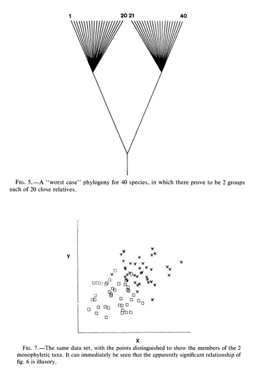
There is a widely held misperception in the scientific community that contrasts regression will sometimes tell us that our observed correlation between traits is spurious - but that the reverse can never be true. That is, that contrasts will not help us to detect evolutionary correlation under circumstances in which correlation is absent or non-significant in the raw data before transformation.

This perception was popularized, perhaps inadvertently, by Felsenstein's (quite accurate) infamous “worst-case scenario”:

Though it is certainly possible that contrasts regression will cause us to conclude that a correlation in the raw data is spurious, (at least theoretically) it is equally plausible that a signficant evolutionary correlation between traits might be revealed by contrasts in circumstances in which none was seen in the original data.

The following is a quick illustration of this that I have used as a 'challenge problem' in my graduate course as well as in some workshops. It uses data that were simulated on a phylogeny under correlated Brownian motion (that is, that are genuinely evolutionarily correlated).

First, load packages:

## load phytools
library(phytools)

Next, we'll read datasets from file. There is nothing magical about these data. The tree was simulated under a stochastic process (admittedly a coalescent rather than pure-birth or birth-death tree, but this is merely to exacerbate the effect of the tree and thus make the point clearer - it would hold in general for any tree shape), and the data were simulated under positively correlated Brownian evolution.

## load data
X<-read.csv("http://www.phytools.org/UMB2015/data/pic-exercise-data.csv",
    row.names=1)
## load tree
tree<-read.tree("http://www.phytools.org/UMB2015/data/pic-exercise-tree.tre")

This is not strictly necessary, but it will make things slightly easier for us moving forward if we pull out the columns of X as separate vectors:

x<-X[,1]
names(x)<-rownames(X)
## or
y<-setNames(X[,2],rownames(X))

Now, let's plot x & y:

plot(x,y)

So, it looks like there is no relationship, right?

fit<-lm(y~x)
plot(x,y)
abline(fit)

fit

## 
## Call:
## lm(formula = y ~ x)
## 
## Coefficients:
## (Intercept)            x  
##    -1.95546     -0.02282

summary(fit)

## 
## Call:
## lm(formula = y ~ x)
## 
## Residuals:
##      Min       1Q   Median       3Q      Max 
## -2.70042 -0.18339  0.04348  0.41484  0.95401 
## 
## Coefficients:
##             Estimate Std. Error t value Pr(>|t|)    
## (Intercept) -1.95546    0.12017 -16.272   <2e-16 ***
## x           -0.02282    0.06582  -0.347     0.73    
## ---
## Signif. codes:  0 '***' 0.001 '**' 0.01 '*' 0.05 '.' 0.1 ' ' 1
## 
## Residual standard error: 0.6289 on 98 degrees of freedom
## Multiple R-squared:  0.001225,   Adjusted R-squared:  -0.008967 
## F-statistic: 0.1202 on 1 and 98 DF,  p-value: 0.7296

anova(fit)

## Analysis of Variance Table
## 
## Response: y
##           Df Sum Sq Mean Sq F value Pr(>F)
## x          1  0.048 0.04753  0.1202 0.7296
## Residuals 98 38.763 0.39554

Now, we take phylogeny into account by computing contrasts:

## compute contrasts
icx<-pic(x,tree)
icy<-pic(y,tree)
## plot contrasts
plot(icx,icy)
## fit model without intercept
fit<-lm(icy~icx-1)
abline(fit)

summary(fit)

## 
## Call:
## lm(formula = icy ~ icx - 1)
## 
## Residuals:
##     Min      1Q  Median      3Q     Max 
## -2.5957 -0.7257  0.2020  0.7100  2.3120 
## 
## Coefficients:
##     Estimate Std. Error t value Pr(>|t|)    
## icx  0.70387    0.09648   7.296 7.81e-11 ***
## ---
## Signif. codes:  0 '***' 0.001 '**' 0.01 '*' 0.05 '.' 0.1 ' ' 1
## 
## Residual standard error: 0.9944 on 98 degrees of freedom
## Multiple R-squared:  0.352,  Adjusted R-squared:  0.3454 
## F-statistic: 53.23 on 1 and 98 DF,  p-value: 7.808e-11

Incredible, right? Our pattern of evolutionary correlation between x & y somehow (seemingly) miraculously appears!

How can we account for this surprising result?

Well, if we project our tree into the phenotype space using a technique called a phylomorphospace plot, we will see that within each clade there is a relationship, but our ability to measure this relationship breaks down due to differences between clades:

phylomorphospace(tree,cbind(x,y),label="off",node.size=c(0,1))

In other words, within clades there is indeed a strongly positive relationship between x & y, but in the raw data this trend is obscured by incidental changes along some of the long internal edges of the tree in a direction contrary to the overall trend of evolution. Note that evolution on these edges was under exactly the same process as it was throughout the rest of the tree, but under a weakly or moderately correlated Brownian process we nonetheless expect that some changes along branches will run contrary to the (average) generating trend, and if these changes happen to occur between clades, then they can obscure the evolutionary pattern when only raw data are examined. Cool.

That's it!